Search icon CANCEL
Subscription
0
Cart icon
Your Cart (0 item)
Close icon
You have no products in your basket yet
Save more on your purchases! discount-offer-chevron-icon
Savings automatically calculated. No voucher code required.
Arrow left icon
Explore Products
Best Sellers
New Releases
Books
Videos
Audiobooks
Learning Hub
Free Learning
Arrow right icon
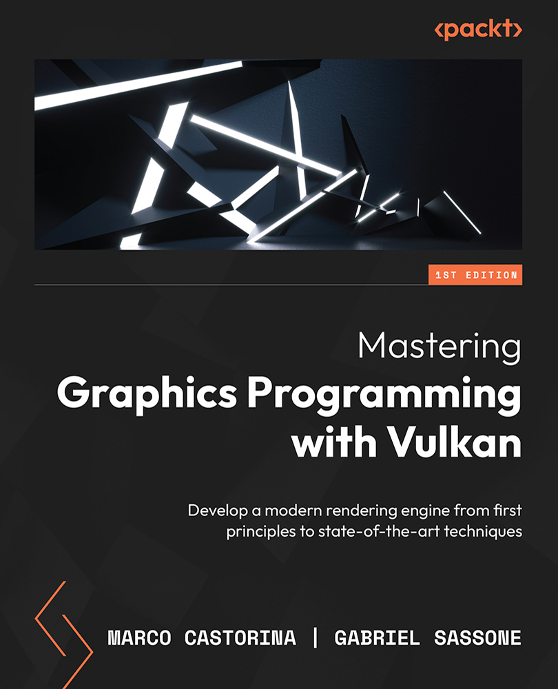
Mastering Graphics Programming with Vulkan

Mastering Graphics Programming with Vulkan: Develop a modern rendering engine from first principles to state-of-the-art techniques

Arrow left icon
Profile Icon Marco Castorina Profile Icon Gabriel Sassone
Arrow right icon
$44.99
Full star icon Full star icon Full star icon Full star icon Half star icon 4.4 (38 Ratings)
Paperback Feb 2023 382 pages 1st Edition
eBook
$9.99 $35.99
Paperback
$44.99
Subscription
Free Trial
Renews at $19.99p/m
eBook
$9.99 $35.99
Paperback
$44.99
Subscription
Free Trial
Renews at $19.99p/m

What do you get with Print?

Product feature icon Instant access to your digital eBook copy whilst your Print order is Shipped
Product feature icon Colour book shipped to your preferred address
Product feature icon Download this book in EPUB and PDF formats
Product feature icon Access this title in our online reader with advanced features
Product feature icon DRM FREE - Read whenever, wherever and however you want
Product feature icon AI Assistant (beta) to help accelerate your learning
OR
Modal Close icon
Payment Processing...
tick Completed

Shipping Address

Billing Address

Shipping Methods
Table of content icon View table of contents Preview book icon Preview Book

Mastering Graphics Programming with Vulkan

Introducing the Raptor Engine and Hydra

When we set out to write this book, we decided our goal was to start where a traditional Vulkan tutorial might end. There are plenty of great resources, both in print and on the web, that help beginners discover and understand the Vulkan API.

We decided to write this book as we felt there was a gap between these introductory tutorials and some of the more advanced material. Some of these topics might be covered in articles and blog posts, but we couldn’t find a resource that organized them in a single and cohesive format.

While we assume some familiarity with Vulkan, in this chapter, we take the opportunity to go over some of the basic concepts that we will build upon throughout the remainder of the book. We will present the code organization and the classes and libraries that we use throughout the book.

In this chapter, we’re going to cover the following main topics:

  • How to read this book
  • Understanding the code structure
  • Understanding the glTF scene format
  • Physically based rendering in a nutshell
  • A word on GPU debugging

By the end of this chapter, you will be familiar with the Raptor Engine and the rendering framework we developed for this book. You will have also learned the structure of the glTF model format and the base concepts behind physically based rendering.

Technical requirements

You will need a GPU that supports at least Vulkan 1.1. At the time of writing, Vulkan 1.3 had just been announced and many vendors, such as AMD and Nvidia, have provided day-one support. We have kept the lower requirements to allow as many people as possible to follow along.

Some of the later chapters will make use of hardware features that might not be available on some of the older graphics cards. Wherever possible, we will provide an alternative software solution. If it’s not feasible, we try to focus more on the generic aspects of the implementation and less on the API details.

The complete code for this chapter is available on GitHub at https://github.com/PacktPublishing/Mastering-Graphics-Programming-with-Vulkan/tree/main/source/chapter1.

Windows

The code has been tested on Windows with Visual Studio 2019 16.11 and the Vulkan SDK version 1.2.198.1 (this might change as we write the book).

To install the Vulkan SDK on Windows, you will need to download and run the following executable:

https://sdk.lunarg.com/sdk/download/1.2.198.1/windows/VulkanSDK-1.2.198.1-Installer.exe

After installing the Vulkan SDK, make sure you can run the vulkaninfoSDK.exe program in the Bin folder to confirm that the SDK has been installed correctly and that your graphics drivers support Vulkan.

Please check the official documentation (https://vulkan.lunarg.com/doc/sdk/latest/windows/getting_started.html) should you need further details on the installation process.

We have provided a Visual Studio solution that contains the full code for the book and that allows you to easily build the executable for each chapter.

Once the solution has been built, set the Chapter1 project as the run target and run the program. Here’s what you should be seeing:

Figure 1.1 – The rendering result

Figure 1.1 – The rendering result

Linux

For Linux, we have used Visual Studio Code, GCC 9 or above, and CMake 3.22.1. The version of the Vulkan SDK matches the one on Windows. We tested both on Debian 11 and Ubuntu 20.04.

We have used CMake to support different build systems, but we have only tested with Makefile.

To install the Vulkan SDK, you will need to download this file: https://sdk.lunarg.com/sdk/download/1.2.198.1/linux/vulkansdk-linux-x86_64-1.2.198.1.tar.gz.

Assuming you have downloaded it in the ~/Downloads folder, extract the package by running the following command:

$ tar -xvf vulkansdk-linux-x86_64-1.2.198.1.tar.gz

This will create the 1.2.198.1 top-level folder.

There are two options to make the SDK available to build the code:

  • You can add the following environment variables to your ~/.bashrc file (or the main configuration file of your shell if you are not using Bash). Please note that you might have to create this file:
    export VULKAN_SDK=~/vulkan/1.2.198.1/x86_64
    export PATH=$VULKAN_SDK/bin:$PATH
    export LD_LIBRARY_PATH=$VULKAN_SDK/lib:
    $LD_LIBRARY_PATH
    export VK_LAYER_PATH=$VULKAN_SDK/etc/vulkan/
    explicit_layer.d
  • The other option is to add the following to your ~/.bashrc file:
    source ~/Downloads/1.2.198.1/setup-env.sh

After you have edited the ~/.bashrc file, restart your Terminal. You should now be able to run vulkaninfo. If that’s not the case, try to follow the previous steps again. Please refer to the official LunarG guide (https://vulkan.lunarg.com/doc/sdk/latest/linux/getting_started.html) should you need more details on the installation process.

To generate the build files, you need to run the following command:

$ cmake -B build -DCMAKE_BUILD_TYPE=Debug

If you’d like to create a release build, run the following command:

$ cmake -B build -DCMAKE_BUILD_TYPE=Release

This will create the build files in the build folder. You can, of course, use a different name for the folder.

To build the code for this chapter, run the following command:

$ cmake --build build --target chapter1 -- -j 4

The number after -j tells the compiler how many threads to use to compile the code in parallel. The recommended value is to use the number of cores your processor has.

After the build has completed, the Chapter1 executable has been created and is ready to run!

Note

Both Windows and Linux builds have been tested throughout the writing of the book by our technical reviewers and beta readers, but some issues might have gone unnoticed. If you have questions or if you would like to report an issue, please open a GitHub issue or reach out to us on Twitter: @marco_castorina and @GabrielSassone.

macOS

Vulkan is not natively available on macOS but is provided through a translation layer into Metal, the graphics API developed by Apple. This translation layer is provided by the Vulkan SDK with the MoltenVK library.

Because of this indirection, not all features and extensions are available on macOS. Given that we are going to make use of some advanced features such as ray tracing in this book, we didn’t want to provide a partially working version of our code for macOS. For the time being, this platform is not supported.

How to read this book

We have organized the content of this book to gradually build on more advanced features. Advanced chapters in this book will rely on topics exposed earlier in the book. For this reason, we suggest that you read the book in order.

However, some of the later chapters on ray tracing could be read in any order as they cover topics that can be developed independently. If you are already familiar with the topic in one of the chapters, we still recommend that you skim through it as you might still find some valuable information.

Understanding the code structure

In this section, we will deep dive into the foundational code used throughout the book and we will explain the rationale behind some of the decisions we made.

When we started thinking about the code to be used, the objective was clear: there was the need for something lightweight, simple, and basic enough to give us the possibility to build upon it. A fully fledged library would have been too much.

Also, we needed something that we were familiar with to make the development process smoother and give us confidence.

There are different great libraries out there, such as Sokol (https://github.com/floooh/sokol) or BGFX (https://github.com/bkaradzic/bgfx), and a few more, but they all have some drawbacks that seemed problematic.

Sokol, for example, even though it is a great library, does not support the Vulkan API, and has an interface still based on older graphics APIs (such as OpenGL and D3D11).

BGFX is a more complete library, but it is a little too generic and feature-fledged to give us the possibility to build upon it.

After some research, we leaned toward the Hydra Engine – a library that Gabriel developed in the last couple of years as code to experiment with and write articles on rendering.

Here are some advantages of starting from the Hydra Engine (https://github.com/JorenJoestar/DataDrivenRendering) and evolving it into the Raptor Engine:

  • Code familiarity
  • Small and simple code base
  • Vulkan-based API
  • No advanced features, but strong building blocks

The Hydra Engine seemed perfect, being small but usable and familiar. From an API design perspective, it was a clear advantage compared to other libraries that both authors had used in the past.

Being designed from scratch by Gabriel, evolving the code through this book is done with the full knowledge of the underlying architecture.

Starting from the Hydra Engine, we changed some code to be more Vulkan-focused, and thus the Raptor Engine was born. In the following sections, we will have a brief look at the code architecture to familiarize you with the building blocks that will be used throughout all the chapters.

We will also look at the glTF data format used to import meshes, textures, and materials into the Raptor Engine.

Layers of code

The Raptor Engine is created with a layer-based mentality for code, in which a layer can interact only with lower ones.

This choice was made to simplify communication between layers and simplify the API design and the expected behavior for the final user.

There are three layers in Raptor:

  • Foundation
  • Graphics
  • Application

The foundation and application layers are common to all chapters and can be found at source/raptor.

Each chapter has its own implementation of the graphics layer. This makes it easier to introduce new features in each chapter without having to worry about maintaining multiple code paths across all chapters. For instance, the code for the graphics layer for this chapter can be found at source/chapter1/graphics.

While developing the Raptor Engine, we enforced the communication direction based on the layer we were on, so that a layer could interact with the code within the same layer and the bottom layer only.

In this case, the foundation layer can interact only with the other code inside the layer, the graphics layer can interact with the foundation layer, and the application layer interacts with all the layers.

There will be possible situations where we need to have some communication from a bottom layer to an upper layer, and the solution to that is to create code in the upper layer to drive the communication between the lower layers.

For example, the Camera class is defined in the foundation layer, and it is a class that contains all the mathematical code to drive a rendering camera.

What if we need user input to move the camera, say with a mouse or gamepad?

Based on this decision, we created GameCamera in the application layer, which contains the input code, takes the user input, and modifies the camera as needed.

This upper layer bridging will be used in other areas of the code and will be explained when needed.

The following sections will give you an overview of the main layers and some of their fundamental code so that you will be familiar with all the available building blocks that will be used throughout the book.

Foundation layer

The foundation layer is a set of different classes that behave as fundamental bricks for everything needed in the framework.

The classes are very specialized and cover different types of needs, but they are required to build the rendering code written in this book. They range from data structures to file operations, logging, and string processing.

While similar data structures are provided by the C++ standard library, we have decided to write our own as we only need a subset of functionality in most cases. It also allows us to carefully control and track memory allocations.

We traded some comfort (that is, automatic release of memory on destruction) for more fine-tuned control over memory lifetime and better compile times. These all-important data structures are used for separate needs and will be used heavily in the graphics layer.

We will briefly go over each foundational block to help you get accustomed to them.

Memory management

Let’s start with memory management (source/raptor/foundation/memory.hpp).

One key API decision made here is to have an explicit allocation model, so for any dynamically allocated memory, an allocator will be needed. This is reflected in all classes through the code base.

This foundational brick defines the main allocator API used by the different allocators that can be used throughout the code.

There is HeapAllocator, based on the tlsf allocator, a fixed-size linear allocator, a malloc-based allocator, a fixed-size stack allocator, and a fixed-size double stack allocator.

While we will not cover memory management techniques here, as it is less relevant to the purpose of this book, you can glimpse a more professional memory management mindset in the code base.

Arrays

Next, we will look at arrays (source/raptor/foundation/array.hpp).

Probably the most fundamental data structure of all software engineering, arrays are used to represent contiguous and dynamically allocated data, with an interface similar to the better-known std::vector (https://en.cppreference.com/w/cpp/container/vector).

The code is simpler compared to the Standard Library (std) implementation and requires an explicit allocator to be initialized.

The only notable difference from std::vector can be seen in the methods, such as push_use(), which grows the array and returns the newly allocated element to be filled, and the delete_swap() method, which removes an element and swaps it with the last element.

Hash maps

Hash maps (source/raptor/foundation/hash_map.hpp) are another fundamental data structure, as they boost search operation performance, and they are used extensively in the code base: every time there is the need to quickly find an object based on some simple search criteria (search the texture by name), then a hash map is the de facto standard data structure.

The sheer volume of information about hash maps is huge and out of the scope of this book, but recently a good all-round implementation of hash maps was documented and shared by Google inside their Abseil library (code available here: https://github.com/abseil/abseil-cpp).

The Abseil hash map is an evolution of the SwissTable hash map, storing some extra metadata per entry to quickly reject elements, using linear probing to insert elements, and finally, using Single Instruction Multiple Data (SIMD) instructions to quickly test more entries.

Important note

For a good overview of the ideas behind the Abseil hash map implementation, there are a couple of nice articles that can be read. They can be found here:

Article 1: https://gankra.github.io/blah/hashbrown-tldr/

Article 2: https://blog.waffles.space/2018/12/07/deep-dive-into-hashbrown/

Article 1 is a good overview of the topic and Article 2 goes a little more in-depth about the implementation.

File operations

Next, we will look at file operations (source/raptor/foundation/file.hpp).

Another common set of operations performed in an engine is file handling, for example, to read a texture, a shader, or a text file from the hard drive.

These operations follow a similar pattern to the C file APIs, such as file_open being similar to the fopen function (https://www.cplusplus.com/reference/cstdio/fopen/).

In this set of functions, there are also the ones needed to create and delete a folder, or some utilities such as extrapolating the filename or the extension of a path.

For example, to create a texture, you need to first open the texture file in memory, then send it to the graphics layer to create a Vulkan representation of it to be properly usable by the GPU.

Serialization

Serialization (source/raptor/foundation/blob_serialization.hpp), the process of converting human-readable files to a binary counterpart, is also present here.

The topic is vast, and there is not as much information as it deserves, but a good starting point is the article https://yave.handmade.network/blog/p/2723-how_media_molecule_does_serialization, or https://jorenjoestar.github.io/post/serialization_for_games.

We will use serialization to process some human-readable files (mostly JSON files) into more custom files as they are needed.

The process is done to speed up loading files, as human-readable formats are great for expressing things and can be modified, but binary files can be created to suit the application’s needs.

This is a fundamental step in any game-related technology, also called asset baking.

For the purpose of this code, we will use a minimal amount of serialization, but as with memory management, it is a topic to have in mind when designing any performant code.

Logging

Logging (source/raptor/foundation/log.hpp) is the process of writing some user-defined text to both help understand the flow of the code and debug the application.

It can be used to write the initialization steps of a system or to report some error with additional information so it can be used by the user.

Provided with the code is a simple logging service, providing the option of adding user-defined callbacks and intercepting any message.

An example of logging usage is the Vulkan debug layer, which will output any warning or error to the logging service when needed, giving the user instantaneous feedback on the application’s behavior.

String processing

Next, we will look at strings (source/raptor/foundation/string.hpp).

Strings are arrays of characters used to store text. Within the Raptor Engine, the need to have clean control of memory and a simple interface added the need for custom-written string code.

The main class provided is the StringBuffer class, which lets the user allocate a maximum fixed amount of memory, and within that memory, perform typical string operations: concatenation, formatting, and substrings.

A second class provided is the StringArray class, which allows the user to efficiently store and track different strings inside a contiguous chunk of memory.

This is used, for example, when retrieving a list of files and folders. A final utility string class is the StringView class, used for read-only access to a string.

Time management

Next is time management (source/raptor/foundation/time.hpp).

When developing a custom engine, timing is very important, and having some functions to help calculate different timings is what the time management functions do.

For example, any application needs to calculate a time difference, used to advance time and calculations in various aspects, often known as delta time.

This will be manually calculated in the application layer, but it uses the time functions to do it. It can be also used to measure CPU performance, for example, to pinpoint slow code or gather statistics when performing some operations.

Timing methods conveniently allow the user to calculate time durations in different units, from seconds down to milliseconds.

Process execution

One last utility area is process execution (source/raptor/foundation/process.hpp) – defined as running any external program from within our own code.

In the Raptor Engine, one of the most important usages of external processes is the execution of Vulkan’s shader compiler to convert GLSL shaders to SPIR-V format, as seen at https://www.khronos.org/registry/SPIR-V/specs/1.0/SPIRV.html. The Khronos specification is needed for shaders to be used by Vulkan.

We have been through all the different utilities building blocks (many seemingly unrelated) that cover the basics of a modern rendering engine.

These basics are not graphics related by themselves, but they are required to build a graphical application that gives the final user full control of what is happening and represents a watered-down mindset of what modern game engines do behind the scenes.

Next, we will introduce the graphics layer, where some of the foundational bricks can be seen in action and represent the most important part of the code base developed for this book.

Graphics layer

The most important architectural layer is the graphics layer, which will be the main focus of this book. Graphics will include all the Vulkan-related code and abstractions needed to draw anything on the screen using the GPU.

There is a caveat in the organization of the source code: having the book divided into different chapters and having one GitHub repository, there was the need to have a snapshot of the graphics code for each chapter; thus, graphics code will be duplicated and evolved in each chapter’s code throughout the game.

We expect the code to grow in this folder as this book progresses after each chapter, and not only here, as we will develop shaders and use other data resources as well, but it is fundamental to know where we are starting from or where we were at a specific time in the book.

Once again, the API design comes from Hydra as follows:

  • Graphics resources are created using a creation struct containing all the necessary parameters
  • Resources are externally passed as handles, so they are easily copiable and safe to pass around

The main class in this layer is the GpuDevice class, which is responsible for the following:

  • Vulkan API abstractions and usage
  • Creation, destruction, and update of graphics resources
  • Swapchain creation, destruction, resize, and update
  • Command buffer requests and submission to the GPU
  • GPU timestamps management
  • GPU-CPU synchronization

We define graphics resources as anything residing on the GPU, such as the following:

  • Textures: Images to read and write from
  • Buffers: Arrays of homogeneous or heterogeneous data
  • Samplers: Converters from raw GPU memory to anything needed from the shaders
  • Shaders: SPIR-V compiled GPU executable code
  • Pipeline: An almost complete snapshot of GPU state

The usage of graphics resources is the core of any type of rendering algorithm.

Therefore, GpuDevice (source/chapter1/graphics/gpu_device.hpp) is the gateway to creating rendering algorithms.

Here is a snippet of the GpuDevice interface for resources:

struct GpuDevice {
  BufferHandle create_buffer( const BufferCreation& bc );
  TextureHandle create_texture( const TextureCreation& tc
  );
  ...
  void destroy_buffer( BufferHandle& handle );
  void destroy_texture( TextureHandle& handle );

Here is an example of the creation and destruction to create VertexBuffer, taken from the Raptor ImGUI (source/chapter1/graphics/raptor_imgui.hpp) backend:

GpuDevice gpu;
// Create the main ImGUI vertex buffer
BufferCreation bc;
bc.set( VK_BUFFER_USAGE_VERTEX_BUFFER_BIT,
  ResourceUsageType::Dynamic, 65536 )
  .set_name( "VB_ImGui" );
BufferHandle imgui_vb = gpu.create(bc);
…
// Destroy the main ImGUI vertex buffer
gpu.destroy(imgui_vb);

In the Raptor Engine, graphics resources (source/chapter1/graphics/gpu_resources.hpp) have the same granularity as Vulkan but are enhanced to help the user write simpler and safer code.

Let’s have a look at the Buffer class:

struct Buffer {
    VkBuffer                        vk_buffer;
    VmaAllocation                   vma_allocation;
    VkDeviceMemory                  vk_device_memory;
    VkDeviceSize                    vk_device_size;
    VkBufferUsageFlags              type_flags      = 0;
    u32                             size            = 0;
    u32                             global_offset   = 0;
    BufferHandle                    handle;
    BufferHandle                    parent_buffer;
    const char* name                = nullptr;
}; // struct Buffer

As we can see, the Buffer struct contains quite a few extra pieces of information.

First of all, VkBuffer is the main Vulkan struct used by the API. Then there are some members related to memory allocations on the GPU, such as device memory and size.

Note that there is a utility class used in the Raptor Engine called Virtual Memory Allocator (VMA) (https://github.com/GPUOpen-LibrariesAndSDKs/VulkanMemoryAllocator), which is the de facto standard utility library to write Vulkan code.

Here, it is reflected in the vma_allocation member variable.

Furthermore, there are usage flags – size and offset, as well as global offsets – current buffer handle and parent handle (we will see their usage later in the book), as well as a human-readable string for easier debugging. This Buffer can be seen as the blueprint of how other abstractions are created in the Raptor Engine, and how they help the user to write simpler and safer code.

They still respect Vulkan’s design and philosophy but can hide some implementation details that can be less important once the focus of the user is exploring rendering algorithms.

We had a brief overview of the graphics layer, the most important part of the code in this book. We will evolve its code after each chapter, and we will dwell deeper on design choices and implementation details throughout the book.

Next, there is the application layer, which works as the final step between the user and the application.

The application layer

The application layer is responsible for handling the actual application side of the engine – from window creation and update based on the operating system to gathering user input from the mouse and keyboard.

In the layer is also included a very handy backend for ImGui (https://github.com/ocornut/imgui), an amazing library to design the UI to enhance user interaction with the application so that it is much easier to control its behavior.

There is an application class that will be the blueprint for any demo application that will be created in the book so that the user can focus more on the graphics side of the application.

The foundation and application layers’ code is in the source/raptor folder. This code will be almost constant throughout the book, but as we are writing mainly a graphics system, this is put in a shared folder between all the chapters.

In this section, we have explained the structure of the code and presented the three main layers of the Raptor Engine: foundation, graphics, and application. For each of these layers, we highlighted some of the main classes, how to use them, and the reasoning and inspiration behind the choices we have made.

In the next section, we are going to present the file format we selected to load 3D data from and how we have integrated it into the engine.

Understanding the glTF scene format

Many 3D file formats have been developed over the years, and for this book, we chose to use glTF. It has become increasingly popular in recent years; it has an open specification, and it supports a physically based rendering (PBR) model by default.

We chose this format because of its open specification and easy-to-understand structure. We can use several models provided by Khronos on GitHub to test our implementation and compare our results with other frameworks.

It is a JSON-based format and we built a custom parser for this book. The JSON data will be deserialized into a C++ class, which we are going to use to drive the rendering.

We now provide an overview of the main sections of the glTF format. At its root, we have a list of scenes, and each scene can have multiple nodes. You can see this in the following code:

"scene": 0,
"scenes": [
    {
        "nodes": [
            0,
            1,
            2,
            3,
            4,
            5
        ]
    }
],

Each node contains an index that is present in the mesh array:

"nodes": [
    {
        "mesh": 0,
        "name": "Hose_low"
    },
]

The data for the scene is stored in one or more buffers, and each section of the buffer is described by a buffer view:

"buffers": [
    {
        "uri": "FlightHelmet.bin",
        "byteLength": 3227148
    }
],
"bufferViews": [
    {
        "buffer": 0,
        "byteLength": 568332,
        "name": "bufferViewScalar"
    },
]

Each buffer view references the buffer that contains the actual data and its size. An accessor points into a buffer view by defining the type, offset, and size of the data:

"accessors": [
    {
        "bufferView": 1,
        "byteOffset": 125664,
        "componentType": 5126,
        "count": 10472,
        "type": "VEC3",
        "name": "accessorNormals"
    }
]

The mesh array contains a list of entries, and each entry is composed of one or more mesh primitives. A mesh primitive contains a list of attributes that point into the accessors array, the index of the indices accessor, and the index of the material:

"meshes": [
    {
        "primitives": [
            {
                "attributes": {
                    "POSITION": 1,
                    "TANGENT": 2,
                    "NORMAL": 3,
                    "TEXCOORD_0": 4
                },
                "indices": 0,
                "material": 0
            }
        ],
        "name": "Hose_low"
    }
]

The materials object defines which textures are used (diffuse color, normal map, roughness, and so on) and other parameters that control the rendering of the material:

"materials": [
    {
        "pbrMetallicRoughness": {
            "baseColorTexture": {
                "index": 2
            },
            "metallicRoughnessTexture": {
                "index": 1
            }
        },
        "normalTexture": {
            "index": 0
        },
        "occlusionTexture": {
            "index": 1
        },
        "doubleSided": true,
        "name": "HoseMat"
    }
]

Each texture is specified as a combination of an image and a sampler:

"textures": [
    {
        "sampler": 0,
        "source": 0,
        "name": "FlightHelmet_Materials_RubberWoodMat_Nor
                 mal.png"
    },
],
"images": [
    {
        "uri": "FlightHelmet_Materials_RubberWoodMat_Nor
                mal.png"
    },
],
"samplers": [
    {
        "magFilter": 9729,
        "minFilter": 9987
    }
]

The glTF format can specify many other details, including animation data and cameras. Most of the models that we are using in this book don’t make use of these features, but we will highlight them when that’s the case.

The JSON data is deserialized into a C++ class, which is then used for rendering. We omitted glTF extensions in the resulting object as they are not used in this book. We are now going through a code example that shows how to read a glTF file using our parser. The first step is to load the file into a glTF object:

char gltf_file[512]{ };
memcpy( gltf_file, argv[ 1 ], strlen( argv[ 1] ) );
file_name_from_path( gltf_file );
glTF::glTF scene = gltf_load_file( gltf_file );

We now have a glTF model loaded into the scene variable.

The next step is to upload the buffers, textures, and samplers that are part of our model to the GPU for rendering. We start by processing textures and samplers:

Array<TextureResource> images;
images.init( allocator, scene.images_count );
for ( u32 image_index = 0; image_index
  < scene.images_count; ++image_index ) {
    glTF::Image& image = scene.images[ image_index ];
    TextureResource* tr = renderer.create_texture(
        image.uri.data, image.uri.data );
    images.push( *tr );
}
Array<SamplerResource> samplers;
samplers.init( allocator, scene.samplers_count );
for ( u32 sampler_index = 0; sampler_index
  < scene.samplers_count; ++sampler_index ) {
  glTF::Sampler& sampler = scene.samplers[ sampler_index ];
  SamplerCreation creation;
  creation.min_filter = sampler.min_filter == glTF::
      Sampler::Filter::LINEAR ? VK_FILTER_LINEAR :
          VK_FILTER_NEAREST;
  creation.mag_filter = sampler.mag_filter == glTF::
      Sampler::Filter::LINEAR ? VK_FILTER_LINEAR :
          VK_FILTER_NEAREST;
  SamplerResource* sr = renderer.create_sampler( creation
  );
  samplers.push( *sr );
}

Each resource is stored in an array. We go through each entry in the array and create the corresponding GPU resource. We then store the resources we just created in a separate array that will be used in the rendering loop.

Now let’s see how we process the buffers and buffer views, as follows:

Array<void*> buffers_data;
buffers_data.init( allocator, scene.buffers_count );
for ( u32 buffer_index = 0; buffer_index
  < scene.buffers_count; ++buffer_index ) {
    glTF::Buffer& buffer = scene.buffers[ buffer_index ];
    FileReadResult buffer_data = file_read_binary(
        buffer.uri.data, allocator );
    buffers_data.push( buffer_data.data );
}
Array<BufferResource> buffers;
buffers.init( allocator, scene.buffer_views_count );
for ( u32 buffer_index = 0; buffer_index
  < scene.buffer_views_count; ++buffer_index ) {
    glTF::BufferView& buffer = scene.buffer_views[
        buffer_index ];
    u8* data = ( u8* )buffers_data[ buffer.buffer ] +
        buffer.byte_offset;
    VkBufferUsageFlags flags =
        VK_BUFFER_USAGE_VERTEX_BUFFER_BIT |
            VK_BUFFER_USAGE_INDEX_BUFFER_BIT;
    BufferResource* br = renderer.create_buffer( flags,
        ResourceUsageType::Immutable, buffer.byte_length,
            data, buffer.name.data );
    buffers.push( *br );
}

First, we read the full buffer data into CPU memory. Then, we iterate through each buffer view and create its corresponding GPU resource. We store the newly created resource in an array that will be used in the rendering loop.

Finally, we read the mesh definition to create its corresponding draw data. The following code provides a sample for reading the position buffer. Please refer to the code in chapter1/main.cpp for the full implementation:

for ( u32 mesh_index = 0; mesh_index < scene.meshes_count;
  ++mesh_index ) {
    glTF::Mesh& mesh = scene.meshes[ mesh_index ];
    glTF::MeshPrimitive& mesh_primitive = mesh.primitives[
        0 ];
    glTF::Accessor& position_accessor = scene.accessors[
        gltf_get_attribute_accessor_index(
        mesh_primitive.attributes, mesh_primitive.
        attribute_count, "POSITION" ) ];
    glTF::BufferView& position_buffer_view =
        scene.buffer_views[ position_accessor.buffer_view
        ];
    BufferResource& position_buffer_gpu = buffers[
        position_accessor.buffer_view ];
    MeshDraw mesh_draw{ };
    mesh_draw.position_buffer = position_buffer_gpu.handle;
    mesh_draw.position_offset = position_accessor.
                                byte_offset;
}

We have grouped all the GPU resources needed to render a mesh into a MeshDraw data structure. We retrieve the buffers and textures as defined by the Accessor object and store them in a MeshDraw object to be used in the rendering loop.

In this chapter, we load a model at the beginning of the application, and it’s not going to change. Thanks to this constraint, we can create all of our descriptor sets only once before we start rendering:

DescriptorSetCreation rl_creation{};
rl_creation.set_layout( cube_rll ).buffer( cube_cb, 0 );
rl_creation.texture_sampler( diffuse_texture_gpu.handle,
    diffuse_sampler_gpu.handle, 1 );
rl_creation.texture_sampler( roughness_texture_gpu.handle,
    roughness_sampler_gpu.handle, 2 );
rl_creation.texture_sampler( normal_texture_gpu.handle,
    normal_sampler_gpu.handle, 3 );
rl_creation.texture_sampler( occlusion_texture_gpu.handle,
    occlusion_sampler_gpu.handle, 4 );
 mesh_draw.descriptor_set = gpu.create_descriptor_set(
     rl_creation );

For each resource type, we call the relative method on the DescriptorSetCreation object. This object stores the data that is going to be used to create the descriptor set through the Vulkan API.

We have now defined all the objects we need for rendering. In our render loop, we simply have to iterate over all meshes, bind each mesh buffer and descriptor set, and call draw:

for ( u32 mesh_index = 0; mesh_index < mesh_draws.size;
  ++mesh_index ) {
    MeshDraw mesh_draw = mesh_draws[ mesh_index ];
    gpu_commands->bind_vertex_buffer( sort_key++,
        mesh_draw.position_buffer, 0,
            mesh_draw.position_offset );
    gpu_commands->bind_vertex_buffer( sort_key++,
        mesh_draw.tangent_buffer, 1,
            mesh_draw.tangent_offset );
    gpu_commands->bind_vertex_buffer( sort_key++,
        mesh_draw.normal_buffer, 2,
            mesh_draw.normal_offset );
    gpu_commands->bind_vertex_buffer( sort_key++,
        mesh_draw.texcoord_buffer, 3,
            mesh_draw.texcoord_offset );
    gpu_commands->bind_index_buffer( sort_key++,
        mesh_draw.index_buffer, mesh_draw.index_offset );
    gpu_commands->bind_descriptor_set( sort_key++,
        &mesh_draw.descriptor_set, 1, nullptr, 0 );
    gpu_commands->draw_indexed( sort_key++,
        TopologyType::Triangle, mesh_draw.count, 1, 0, 0,
            0 );
}

We are going to evolve this code over the course of the book, but it’s already a great starting point for you to try and load a different model or to experiment with the shader code (more on this in the next section).

There are several tutorials online about the glTF format, some of which are linked in the Further reading section. The glTF spec is also a great source of details and is easy to follow. We recommend you refer to it if something about the format is not immediately clear from reading the book or the code.

In this section, we have analyzed the glTF format and we have presented examples of the JSON objects most relevant to our renderer. We then demonstrated how to use the glTF parser, which we added to our framework, and showed you how to upload geometry and texture data to the GPU. Finally, we have shown how to use this data to draw the meshes that make up a model.

In the next section, we explain how the data we just parsed and uploaded to the GPU is used to render our model using a physically-based rendering implementation.

PBR in a nutshell

PBR is at the heart of many rendering engines. It was originally developed for offline rendering, but thanks to the advances in hardware capabilities and research efforts by the graphics community, it can now be used for real-time rendering as well.

As the name implies, this technique aims at modeling the physical interactions of light and matter and, in some implementations, ensuring that the amount of energy in the system is preserved.

There are plenty of in-depth resources available that describe PBR in great detail. Nonetheless, we want to give a brief overview of our implementation for reference. We have followed the implementation presented in the glTF spec.

To compute the final color of our surface, we have to determine the diffuse and specular components. The amount of specular reflection in the real world is determined by the roughness of the surface. The smoother the surface, the greater the amount of light that is reflected. A mirror reflects (almost) all the light it receives.

The roughness of the surface is modeled through a texture. In the glTF format, this value is packed with the metalness and the occlusion values in a single texture to optimize resource use. We distinguish materials between conductors (or metallic) and dielectric (non-metallic) surfaces.

A metallic material has only a specular term, while a non-metallic material has both diffuse and specular terms. To model materials that have both metallic and non-metallic components, we use the metalness term to interpolate between the two.

An object made of wood will likely have a metalness of 0, plastic will have a mix of both metalness and roughness, and the body of a car will be dominated by the metallic component.

As we are modeling the real-world response of a material, we need a function that takes the view and light direction and returns the amount of light that is reflected. This function is called the bi-directional distribution function (BRDF).

We use the Trowbridge-Reitz/GGX distribution for the specular BRDF, and it is implemented as follows:

float NdotH = dot(N, H);
float alpha_squared = alpha * alpha;
float d_denom = ( NdotH * NdotH ) * ( alpha_squared - 1.0 )
    + 1.0;
float distribution = ( alpha_squared * heaviside( NdotH ) )
    / ( PI * d_denom * d_denom );
float NdotL = dot(N, L);
float NdotV = dot(N, V);
float HdotL = dot(H, L);
float HdotV = dot(H, V);
float visibility = ( heaviside( HdotL ) / ( abs( NdotL ) +
  sqrt( alpha_squared + ( 1.0 - alpha_squared ) *
  ( NdotL * NdotL ) ) ) ) * ( heaviside( HdotV ) /
  ( abs( NdotV ) + sqrt( alpha_squared +
  ( 1.0 - alpha_squared ) *
  ( NdotV * NdotV ) ) ) );
float specular_brdf = visibility * distribution;

First, we compute the distribution and visibility terms according to the formula presented in the glTF specification. Then, we multiply them to obtain the specular BRDF term.

There are other approximations that can be used, and we encourage you to experiment and replace ours with a different one!

We then compute the diffuse BDRF, as follows:

vec3 diffuse_brdf = (1 / PI) * base_colour.rgb;

We now introduce the Fresnel term. This determines the color of the reflection based on the viewing angle and the index of refraction of the material. Here is the implementation of the Schlick approximation, both for the metallic and dielectric components:

// f0 in the formula notation refers to the base colour
   here
vec3 conductor_fresnel = specular_brdf * ( base_colour.rgb
  + ( 1.0 - base_colour.rgb ) * pow( 1.0 - abs( HdotV ),
      5 ) );
// f0 in the formula notation refers to the value derived
   from ior = 1.5
float f0 = 0.04; // pow( ( 1 - ior ) / ( 1 + ior ), 2 )
float fr = f0 + ( 1 - f0 ) * pow(1 - abs( HdotV ), 5 );
vec3 fresnel_mix = mix( diffuse_brdf, vec3(
                        specular_brdf ), fr );

Here we compute the Fresnel term for both the conductor and the dielectric components according to the formula in the glTF specification.

Now that we have computed all the components of the model, we interpolate between them, based on the metalness of the material, as follows:

vec3 material_colour = mix( resnel_mix,
                            conductor_fresnel, metalness );

The occlusion term is not used as it only affects indirect light, which we haven’t implemented yet.

We realize this is a very quick introduction, and we skipped over a lot of the theory that makes these approximations work. However, it should provide a good starting point for further study.

We have added links to some excellent resources in the Further reading section if you’d like to experiment and modify our base implementation.

In the next section, we are going to introduce a debugging tool that we rely on whenever we have a non-trivial rendering issue. It has helped us many times while writing this book!

A word on GPU debugging

No matter how much experience you have in graphics programming, there will come a time when you need to debug an issue. Understanding exactly what the GPU is doing when it executes your program is not as immediate as on the CPU. Thankfully, GPU debugging tools have come a long way to help us when our program doesn’t behave as expected.

GPU vendors provide great tools to debug and profile your shaders: Nvidia has developed Nsight graphics, and AMD has a suite of tools that includes the Radeon GPU analyzer and Radeon GPU profiler.

For this book, we have primarily used RenderDoc (available at https://renderdoc.org/). It is a staple tool of the graphics programming community as it allows you to capture a frame and record all the Vulkan API calls that have been issued during that frame.

Using RenderDoc is really simple. You start by providing the path to your application, as follows:

Figure 1.2 – Setting the application path in RenderDoc

Figure 1.2 – Setting the application path in RenderDoc

You then start the application by clicking Launch, and you will notice an overlay reporting the frame time and the number of frames rendered. If you press F12, RenderDoc will record the current frame. You can now close your application, and the recorded frame will automatically load.

On the left, you have the list of API calls grouped in render passes. This view also lists the event ID (EID), which is a progressive number defined by RenderDoc. This is useful for comparing events across multiple frames:

Figure 1.3 – The list of Vulkan API calls for the captured frame

Figure 1.3 – The list of Vulkan API calls for the captured frame

On the right side of the application window, you have multiple tabs that allow you to inspect which textures are bound when a draw call is made, the buffer content, and the state of the pipeline.

The following figure shows the Texture Viewer tab. It shows the rendering output after a given draw and which input textures were bound:

Figure 1.4 – RenderDoc texture viewer

Figure 1.4 – RenderDoc texture viewer

If you right-click on a pixel in the Texture Viewer tab, you can inspect the history of that pixel to understand which draws affected it.

There is also a debug feature that allows you to step through the shader code and analyze intermediate values. Be careful when using this feature, as we have noticed that the values are not always accurate.

This was a quick overview of RenderDoc and its functionality. You have learned how to capture a frame in RenderDoc when running a graphics application. We presented a breakdown of the main panels, their functionality, and how to use them to understand how the final image is rendered.

We encourage you to run the code from this chapter under RenderDoc to better understand how the frame is built.

Summary

In this chapter, we laid the foundations for the rest of the book. By now, you should be familiar with how the code is structured and how to use it. We introduced the Raptor Engine, and we have provided an overview of the main classes and libraries that are going to be used throughout the book.

We have presented the glTF format of the 3D models and how we parse this format into objects that will be used for rendering. We gave a brief introduction to PBR modeling and our implementation of it. Finally, we introduced RenderDoc and how it can be used to debug rendering issues or to understand how a frame is built.

In the next chapter, we are going to look at how to improve our resource management!

Further reading

We have only skimmed the surface of the topics we have presented. Here, we provide links to resources you can use to get more information on the concepts exposed in this chapter, which will be useful throughout the book.

While we have written our own standard library replacement, there are other options if you are starting your own project. We highly recommend looking into https://github.com/electronicarts/EASTL, developed by EA.

Left arrow icon Right arrow icon
Download code icon Download Code

Key benefits

  • Use a pre-built "Raptor" engine to abstract tedious aspects like file systems, memory allocation, and utility functions
  • Delve into advanced graphics programming by taking advantage of Vulkan's cutting-edge features, including mesh shaders and ray tracing
  • Optimize your engine without reinventing the wheel
  • Purchase of the print or Kindle book includes a free PDF eBook

Description

Vulkan is now an established and flexible multi-platform graphics API. It has been adopted in many industries, including game development, medical imaging, movie productions, and media playback but learning it can be a daunting challenge due to its low-level, complex nature. Mastering Graphics Programming with Vulkan is designed to help you overcome this difficulty, providing a practical approach to learning one of the most advanced graphics APIs. In Mastering Graphics Programming with Vulkan, you’ll focus on building a high-performance rendering engine from the ground up. You’ll explore Vulkan’s advanced features, such as pipeline layouts, resource barriers, and GPU-driven rendering, to automate tedious tasks and create efficient workflows. Additionally, you'll delve into cutting-edge techniques like mesh shaders and real-time ray tracing, elevating your graphics programming to the next level. By the end of this book, you’ll have a thorough understanding of modern rendering engines to confidently handle large-scale projects. Whether you're developing games, simulations, or visual effects, this guide will equip you with the skills and knowledge to harness Vulkan’s full potential.

Who is this book for?

This book is for professional graphics and game developers who want to gain in-depth knowledge about how to write a modern and performant rendering engine in Vulkan. Familiarity with basic concepts of graphics programming (i.e. matrices, vectors, etc.) and fundamental knowledge of Vulkan are required.

What you will learn

  • Understand resources management and modern bindless techniques
  • Get comfortable with how a frame graph works and know its advantages
  • Explore how to render efficiently with many light sources
  • Discover how to integrate variable rate shading
  • Understand the benefits and limitations of temporal anti-aliasing
  • Get to grips with how GPU-driven rendering works
  • Explore and leverage ray tracing to improve render quality
Estimated delivery fee Deliver to United States

Economy delivery 10 - 13 business days

Free $6.95

Premium delivery 6 - 9 business days

$21.95
(Includes tracking information)

Product Details

Country selected
Publication date, Length, Edition, Language, ISBN-13
Publication date : Feb 10, 2023
Length: 382 pages
Edition : 1st
Language : English
ISBN-13 : 9781803244792
Languages :
Tools :

What do you get with Print?

Product feature icon Instant access to your digital eBook copy whilst your Print order is Shipped
Product feature icon Colour book shipped to your preferred address
Product feature icon Download this book in EPUB and PDF formats
Product feature icon Access this title in our online reader with advanced features
Product feature icon DRM FREE - Read whenever, wherever and however you want
Product feature icon AI Assistant (beta) to help accelerate your learning
OR
Modal Close icon
Payment Processing...
tick Completed

Shipping Address

Billing Address

Shipping Methods
Estimated delivery fee Deliver to United States

Economy delivery 10 - 13 business days

Free $6.95

Premium delivery 6 - 9 business days

$21.95
(Includes tracking information)

Product Details

Publication date : Feb 10, 2023
Length: 382 pages
Edition : 1st
Language : English
ISBN-13 : 9781803244792
Languages :
Tools :

Packt Subscriptions

See our plans and pricing
Modal Close icon
$19.99 billed monthly
Feature tick icon Unlimited access to Packt's library of 7,000+ practical books and videos
Feature tick icon Constantly refreshed with 50+ new titles a month
Feature tick icon Exclusive Early access to books as they're written
Feature tick icon Solve problems while you work with advanced search and reference features
Feature tick icon Offline reading on the mobile app
Feature tick icon Simple pricing, no contract
$199.99 billed annually
Feature tick icon Unlimited access to Packt's library of 7,000+ practical books and videos
Feature tick icon Constantly refreshed with 50+ new titles a month
Feature tick icon Exclusive Early access to books as they're written
Feature tick icon Solve problems while you work with advanced search and reference features
Feature tick icon Offline reading on the mobile app
Feature tick icon Choose a DRM-free eBook or Video every month to keep
Feature tick icon PLUS own as many other DRM-free eBooks or Videos as you like for just $5 each
Feature tick icon Exclusive print discounts
$279.99 billed in 18 months
Feature tick icon Unlimited access to Packt's library of 7,000+ practical books and videos
Feature tick icon Constantly refreshed with 50+ new titles a month
Feature tick icon Exclusive Early access to books as they're written
Feature tick icon Solve problems while you work with advanced search and reference features
Feature tick icon Offline reading on the mobile app
Feature tick icon Choose a DRM-free eBook or Video every month to keep
Feature tick icon PLUS own as many other DRM-free eBooks or Videos as you like for just $5 each
Feature tick icon Exclusive print discounts

Frequently bought together


Stars icon
Total $ 149.97
Mastering Graphics Programming with Vulkan
$44.99
Mathematics for Game Programming and Computer Graphics
$54.99
C++ Game Animation Programming
$49.99
Total $ 149.97 Stars icon
Banner background image

Table of Contents

20 Chapters
Part 1: Foundations of a Modern Rendering Engine Chevron down icon Chevron up icon
Chapter 1: Introducing the Raptor Engine and Hydra Chevron down icon Chevron up icon
Chapter 2: Improving Resources Management Chevron down icon Chevron up icon
Chapter 3: Unlocking Multi-Threading Chevron down icon Chevron up icon
Chapter 4: Implementing a Frame Graph Chevron down icon Chevron up icon
Chapter 5: Unlocking Async Compute Chevron down icon Chevron up icon
Part 2: GPU-Driven Rendering Chevron down icon Chevron up icon
Chapter 6: GPU-Driven Rendering Chevron down icon Chevron up icon
Chapter 7: Rendering Many Lights with Clustered Deferred Rendering Chevron down icon Chevron up icon
Chapter 8: Adding Shadows Using Mesh Shaders Chevron down icon Chevron up icon
Chapter 9: Implementing Variable Rate Shading Chevron down icon Chevron up icon
Chapter 10: Adding Volumetric Fog Chevron down icon Chevron up icon
Part 3: Advanced Rendering Techniques Chevron down icon Chevron up icon
Chapter 11: Temporal Anti-Aliasing Chevron down icon Chevron up icon
Chapter 12: Getting Started with Ray Tracing Chevron down icon Chevron up icon
Chapter 13: Revisiting Shadows with Ray Tracing Chevron down icon Chevron up icon
Chapter 14: Adding Dynamic Diffuse Global Illumination with Ray Tracing Chevron down icon Chevron up icon
Chapter 15: Adding Reflections with Ray Tracing Chevron down icon Chevron up icon
Index Chevron down icon Chevron up icon
Other Books You May Enjoy Chevron down icon Chevron up icon

Customer reviews

Top Reviews
Rating distribution
Full star icon Full star icon Full star icon Full star icon Half star icon 4.4
(38 Ratings)
5 star 68.4%
4 star 18.4%
3 star 5.3%
2 star 5.3%
1 star 2.6%
Filter icon Filter
Top Reviews

Filter reviews by


Salim Pamukcu Feb 06, 2024
Full star icon Full star icon Full star icon Full star icon Full star icon 5
this is an excellent book which you understanding from the beginning ; including the build systems, how to get the drivers and very useful information that can be used if you are dealing with Vulkan Api
Feefo Verified review Feefo
N/A Jun 01, 2024
Full star icon Full star icon Full star icon Full star icon Full star icon 5
Very well explained with good examples and useful code.
Feefo Verified review Feefo
Andreia G. Feb 13, 2023
Full star icon Full star icon Full star icon Full star icon Full star icon 5
This is a great Vulkan resource, concise and straightforward, aggregating a ton of information that you might have to dig around in random corners of the internet all in one place. The code snippets are well done, readable and very approachable, and the whole book follows a natural progression of practical usage of modern Vulkan.The use of a custom engine as a basis to show how Vulkan works is a really good idea! It provides a lot of context - Vulkan is very broad and can be used in a million ways, so having a concrete project and framework to focus on works very well. I'll be referring back to this book a lot in my Vulkan adventures!
Amazon Verified review Amazon
Omid May 03, 2024
Full star icon Full star icon Full star icon Full star icon Full star icon 5
On my first read i was dissapointed that it is not really a "vulkan" book. The last few chapters don't even mention vulkan api at all. However, once I started rereading it just as a graphics programming guide, i realized this is an amazing book. Going step by step through how to implement various techniques is much more valuable than just showing how to master a graphics api. Hopefully they'll come up with a 2nd edition with even more recent techniques like restir.
Amazon Verified review Amazon
Martin Valigursky Feb 10, 2023
Full star icon Full star icon Full star icon Full star icon Full star icon 5
The books looks at many modern rendering techniques. Its starts with the introduction of core techniques modern engines use, and explains details on how to use them and integrate them into the engine. Things like multi-threaded command buffer recording, frame graph using resource allocation / sharing, using of compute shaders. It builds on these to build a core rendering engine using meshlets, while doing culling on the GPU. Clustered lighting is used to effectively add large number of lights to the scene, most of which is running completely on the GPU.One of my favorite parts was the chapter on the temporal antialiasing, as that is something I'm keen to add to my engine. I enjoyed that the book starts with the simplest implementation that is reasonably easy to implement, and builds multiple improvement levels on top of this.Few last chapters are given to ray tracking, starting with overview of how raytracing fits into to the rendering pipeline and shaders. Then it explained implementation of multiple advanced topics, such as soft shadows, global illumination, and reflections. I have not used raytracing yet, so I was very eager to learn about this.Another thing I enjoyed is a list of references to many papers / websites and tutorials to help one with more detailed understanding of the topics discussed. This are part of every chapter, making it easy to access. The book typically gives you only a reasonably minimal introduction to some of these topics, before it focuses on the actual implementation, and so it's great to have additional resources handy if you're interested in more details.Overall, this was a very enjoyable read, an I'll be referencing the book and the resources it provides while I add many features to my engine!
Amazon Verified review Amazon
Get free access to Packt library with over 7500+ books and video courses for 7 days!
Start Free Trial

FAQs

What is the delivery time and cost of print book? Chevron down icon Chevron up icon

Shipping Details

USA:

'

Economy: Delivery to most addresses in the US within 10-15 business days

Premium: Trackable Delivery to most addresses in the US within 3-8 business days

UK:

Economy: Delivery to most addresses in the U.K. within 7-9 business days.
Shipments are not trackable

Premium: Trackable delivery to most addresses in the U.K. within 3-4 business days!
Add one extra business day for deliveries to Northern Ireland and Scottish Highlands and islands

EU:

Premium: Trackable delivery to most EU destinations within 4-9 business days.

Australia:

Economy: Can deliver to P. O. Boxes and private residences.
Trackable service with delivery to addresses in Australia only.
Delivery time ranges from 7-9 business days for VIC and 8-10 business days for Interstate metro
Delivery time is up to 15 business days for remote areas of WA, NT & QLD.

Premium: Delivery to addresses in Australia only
Trackable delivery to most P. O. Boxes and private residences in Australia within 4-5 days based on the distance to a destination following dispatch.

India:

Premium: Delivery to most Indian addresses within 5-6 business days

Rest of the World:

Premium: Countries in the American continent: Trackable delivery to most countries within 4-7 business days

Asia:

Premium: Delivery to most Asian addresses within 5-9 business days

Disclaimer:
All orders received before 5 PM U.K time would start printing from the next business day. So the estimated delivery times start from the next day as well. Orders received after 5 PM U.K time (in our internal systems) on a business day or anytime on the weekend will begin printing the second to next business day. For example, an order placed at 11 AM today will begin printing tomorrow, whereas an order placed at 9 PM tonight will begin printing the day after tomorrow.


Unfortunately, due to several restrictions, we are unable to ship to the following countries:

  1. Afghanistan
  2. American Samoa
  3. Belarus
  4. Brunei Darussalam
  5. Central African Republic
  6. The Democratic Republic of Congo
  7. Eritrea
  8. Guinea-bissau
  9. Iran
  10. Lebanon
  11. Libiya Arab Jamahriya
  12. Somalia
  13. Sudan
  14. Russian Federation
  15. Syrian Arab Republic
  16. Ukraine
  17. Venezuela
What is custom duty/charge? Chevron down icon Chevron up icon

Customs duty are charges levied on goods when they cross international borders. It is a tax that is imposed on imported goods. These duties are charged by special authorities and bodies created by local governments and are meant to protect local industries, economies, and businesses.

Do I have to pay customs charges for the print book order? Chevron down icon Chevron up icon

The orders shipped to the countries that are listed under EU27 will not bear custom charges. They are paid by Packt as part of the order.

List of EU27 countries: www.gov.uk/eu-eea:

A custom duty or localized taxes may be applicable on the shipment and would be charged by the recipient country outside of the EU27 which should be paid by the customer and these duties are not included in the shipping charges been charged on the order.

How do I know my custom duty charges? Chevron down icon Chevron up icon

The amount of duty payable varies greatly depending on the imported goods, the country of origin and several other factors like the total invoice amount or dimensions like weight, and other such criteria applicable in your country.

For example:

  • If you live in Mexico, and the declared value of your ordered items is over $ 50, for you to receive a package, you will have to pay additional import tax of 19% which will be $ 9.50 to the courier service.
  • Whereas if you live in Turkey, and the declared value of your ordered items is over € 22, for you to receive a package, you will have to pay additional import tax of 18% which will be € 3.96 to the courier service.
How can I cancel my order? Chevron down icon Chevron up icon

Cancellation Policy for Published Printed Books:

You can cancel any order within 1 hour of placing the order. Simply contact customercare@packt.com with your order details or payment transaction id. If your order has already started the shipment process, we will do our best to stop it. However, if it is already on the way to you then when you receive it, you can contact us at customercare@packt.com using the returns and refund process.

Please understand that Packt Publishing cannot provide refunds or cancel any order except for the cases described in our Return Policy (i.e. Packt Publishing agrees to replace your printed book because it arrives damaged or material defect in book), Packt Publishing will not accept returns.

What is your returns and refunds policy? Chevron down icon Chevron up icon

Return Policy:

We want you to be happy with your purchase from Packtpub.com. We will not hassle you with returning print books to us. If the print book you receive from us is incorrect, damaged, doesn't work or is unacceptably late, please contact Customer Relations Team on customercare@packt.com with the order number and issue details as explained below:

  1. If you ordered (eBook, Video or Print Book) incorrectly or accidentally, please contact Customer Relations Team on customercare@packt.com within one hour of placing the order and we will replace/refund you the item cost.
  2. Sadly, if your eBook or Video file is faulty or a fault occurs during the eBook or Video being made available to you, i.e. during download then you should contact Customer Relations Team within 14 days of purchase on customercare@packt.com who will be able to resolve this issue for you.
  3. You will have a choice of replacement or refund of the problem items.(damaged, defective or incorrect)
  4. Once Customer Care Team confirms that you will be refunded, you should receive the refund within 10 to 12 working days.
  5. If you are only requesting a refund of one book from a multiple order, then we will refund you the appropriate single item.
  6. Where the items were shipped under a free shipping offer, there will be no shipping costs to refund.

On the off chance your printed book arrives damaged, with book material defect, contact our Customer Relation Team on customercare@packt.com within 14 days of receipt of the book with appropriate evidence of damage and we will work with you to secure a replacement copy, if necessary. Please note that each printed book you order from us is individually made by Packt's professional book-printing partner which is on a print-on-demand basis.

What tax is charged? Chevron down icon Chevron up icon

Currently, no tax is charged on the purchase of any print book (subject to change based on the laws and regulations). A localized VAT fee is charged only to our European and UK customers on eBooks, Video and subscriptions that they buy. GST is charged to Indian customers for eBooks and video purchases.

What payment methods can I use? Chevron down icon Chevron up icon

You can pay with the following card types:

  1. Visa Debit
  2. Visa Credit
  3. MasterCard
  4. PayPal
What is the delivery time and cost of print books? Chevron down icon Chevron up icon

Shipping Details

USA:

'

Economy: Delivery to most addresses in the US within 10-15 business days

Premium: Trackable Delivery to most addresses in the US within 3-8 business days

UK:

Economy: Delivery to most addresses in the U.K. within 7-9 business days.
Shipments are not trackable

Premium: Trackable delivery to most addresses in the U.K. within 3-4 business days!
Add one extra business day for deliveries to Northern Ireland and Scottish Highlands and islands

EU:

Premium: Trackable delivery to most EU destinations within 4-9 business days.

Australia:

Economy: Can deliver to P. O. Boxes and private residences.
Trackable service with delivery to addresses in Australia only.
Delivery time ranges from 7-9 business days for VIC and 8-10 business days for Interstate metro
Delivery time is up to 15 business days for remote areas of WA, NT & QLD.

Premium: Delivery to addresses in Australia only
Trackable delivery to most P. O. Boxes and private residences in Australia within 4-5 days based on the distance to a destination following dispatch.

India:

Premium: Delivery to most Indian addresses within 5-6 business days

Rest of the World:

Premium: Countries in the American continent: Trackable delivery to most countries within 4-7 business days

Asia:

Premium: Delivery to most Asian addresses within 5-9 business days

Disclaimer:
All orders received before 5 PM U.K time would start printing from the next business day. So the estimated delivery times start from the next day as well. Orders received after 5 PM U.K time (in our internal systems) on a business day or anytime on the weekend will begin printing the second to next business day. For example, an order placed at 11 AM today will begin printing tomorrow, whereas an order placed at 9 PM tonight will begin printing the day after tomorrow.


Unfortunately, due to several restrictions, we are unable to ship to the following countries:

  1. Afghanistan
  2. American Samoa
  3. Belarus
  4. Brunei Darussalam
  5. Central African Republic
  6. The Democratic Republic of Congo
  7. Eritrea
  8. Guinea-bissau
  9. Iran
  10. Lebanon
  11. Libiya Arab Jamahriya
  12. Somalia
  13. Sudan
  14. Russian Federation
  15. Syrian Arab Republic
  16. Ukraine
  17. Venezuela