Search icon CANCEL
Subscription
0
Cart icon
Your Cart (0 item)
Close icon
You have no products in your basket yet
Arrow left icon
Explore Products
Best Sellers
New Releases
Books
Videos
Audiobooks
Learning Hub
Conferences
Free Learning
Arrow right icon
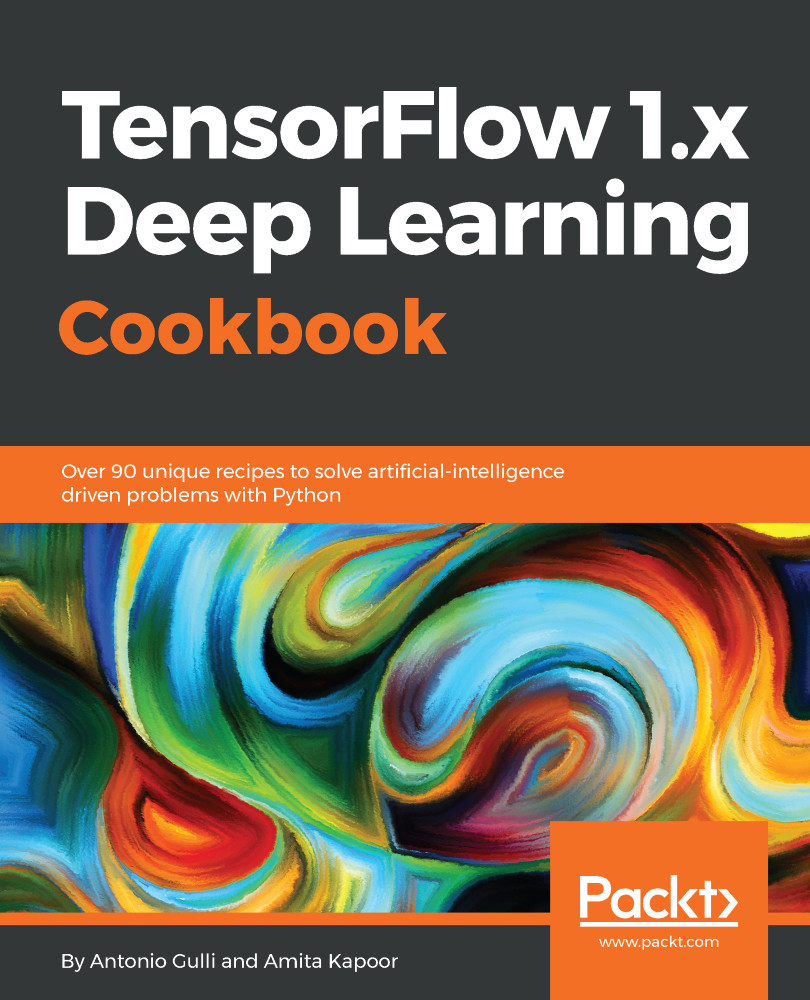
TensorFlow 1.x Deep Learning Cookbook

TensorFlow 1.x Deep Learning Cookbook: Over 90 unique recipes to solve artificial-intelligence driven problems with Python

eBook
€8.99 €29.99
Paperback
€36.99
Subscription
Free Trial
Renews at €18.99p/m

What do you get with Print?

Product feature icon Instant access to your digital eBook copy whilst your Print order is Shipped
Product feature icon Paperback book shipped to your preferred address
Product feature icon Download this book in EPUB and PDF formats
Product feature icon Access this title in our online reader with advanced features
Product feature icon DRM FREE - Read whenever, wherever and however you want
OR
Modal Close icon
Payment Processing...
tick Completed

Shipping Address

Billing Address

Shipping Methods
Table of content icon View table of contents Preview book icon Preview Book

TensorFlow 1.x Deep Learning Cookbook

TensorFlow - An Introduction

Anyone who has ever tried to write code for neural networks in Python using only NumPy, knows how cumbersome it is. Writing code for a simple one-layer feedforward network requires more than 40 lines, made more difficult as you add the number of layers both in terms of writing code and execution time.

TensorFlow makes it all easier and faster reducing the time between the implementation of an idea and deployment. In this book, you will learn how to unravel the power of TensorFlow to implement deep neural networks.

In this chapter, we will cover the following topics:

  • Installing TensorFlow
  • Hello world in TensorFlow
  • Understanding the TensorFlow program structure
  • Working with constants, variables, and placeholders
  • Performing matrix manipulations using TensorFlow
  • Using a data flow graph
  • Migrating from 0.x to 1.x
  • Using XLA to enhance computational performance
  • Invoking CPU/GPU devices
  • TensorFlow for deep learning
  • Different Python packages required for DNN-based problems

Introduction

TensorFlow is a powerful open source software library developed by the Google Brain team for deep neural networks (DNNs). It was first made available under the Apache 2.x License in November 2015; as of today, its GitHub repository (https://github.com/tensorflow/tensorflow) has more than 17,000 commits, with roughly 845 contributors in just two years. This by itself is a measure of both the popularity and performance of TensorFlow. The following graph shows a comparison of the popular deep learning frameworks where it is clearly visible that TensorFlow is the leader among them:

The Figure is based on data taken from the Github repositories of each as on 12 July 2017. Each Bubble has a legend: (Framework, contributors).

Let's first learn what exactly TensorFlow is and why is it so popular among DNN researchers and engineers. TensorFlow, the open source deep learning library allows one to deploy deep neural networks computation on one or more CPU, GPUs in a server, desktop or mobile using the single TensorFlow API. You might ask, there are so many other deep learning libraries such as Torch, Theano, Caffe, and MxNet; what makes TensorFlow special? Most of other deep learning libraries like TensorFlow have auto-differentiation, many are open source, most support CPU/GPU options, have pretrained models, and support commonly used NN architectures like recurrent neural networks (RNNs), convolutional neural networks (CNNs), and deep belief networks (DBNs). So, what more is there in TensorFlow? Let's list them for you:

  • It works with all the cool languages. TensorFlow works with Python, C++, Java, R, and Go.
  • TensorFlow works on multiple platforms, even mobile and distributed.
  • It is supported by all cloud providers--AWS, Google, and Azure.
  • Keras, a high-level neural network API, has been integrated with TensorFlow.
  • It has better computational graph visualizations because it is native while the equivalent in Torch/Theano is not nearly as cool to look at.
  • TensorFlow allows model deployment and ease of use in production.
  • TensorFlow has very good community support.
  • TensorFlow is more than a software library; it is a suite of software that includes TensorFlow, TensorBoard, and TensorServing.

The Google research blog (https://research.googleblog.com/2016/11/celebrating-tensorflows-first-year.html) lists some of the fascinating projects done by people around the world using TensorFlow:

  • Google Translate is using TensorFlow and tensor processing units (TPUs)
  • Project Magenta, which can produce melodies using reinforcement learning-based models, employs TensorFlow
  • Australian marine biologists are using TensorFlow to find and understand sea-cows, which are on the verge of extinction
  • A Japanese farmer used TensorFlow to develop an application to sort cucumbers using physical parameters like size and shape

The list is long, and the possibilities in which one can use TensorFlow are even greater. This book aims to provide you with an understanding of TensorFlow as applied to deep learning models such that you can adapt them to your dataset with ease and develop useful applications. Each chapter contains a set of recipes which deal with the technical issues, the dependencies, the actual code, and its understanding. We have built the recipes one on another such that, by the end of each chapter, you have a fully functional deep learning model.

Installing TensorFlow

In this recipe, you will learn how to do a fresh installation of TensorFlow 1.3 on different OSes (Linux, Mac, and Windows). We will find out about the necessary requirements to install TensorFlow. TensorFlow can be installed using native pip, Anaconda, virtualenv, and Docker on Ubuntu and macOS. For Windows OS, one can use native pip or Anaconda.

As Anaconda works on all the three OSes and provides an easy way to not only install but also to maintain different project environments on the same system, we will concentrate on installing TensorFlow using Anaconda in this book. More details about Anaconda and managing its environment can be read from https://conda.io/docs/user-guide/index.html.

The code in this book has been tested on the following platforms:

  • Windows 10, Anaconda 3, Python 3.5, TensorFlow GPU, CUDA toolkit 8.0, cuDNN v5.1, NVDIA® GTX 1070
  • Windows 10/ Ubuntu 14.04/ Ubuntu 16.04/macOS Sierra, Anaconda3, Python 3.5, TensorFlow (CPU)

Getting ready

The prerequisite for TensorFlow installation is that the system has Python 2.5 or higher installed. The recipes in this book have been designed for Python 3.5 (the Anaconda 3 distribution). To get ready for the installation of TensorFlow, first ensure that you have Anaconda installed. You can download and install Anaconda for Windows/macOS or Linux from https://www.continuum.io/downloads.

After installation, you can verify the installation using the following command in your terminal window:

conda --version

Once Anaconda is installed, we move to the next step, deciding whether to install TensorFlow CPU or GPU. While almost all computer machines support TensorFlow CPU, TensorFlow GPU can be installed only if the machine has an NVDIA® GPU card with CUDA compute capability 3.0 or higher (minimum NVDIA® GTX 650 for desktop PCs).

CPU versus GPU: Central Processing Unit (CPU) consists of a few cores (4-8) optimized for sequential serial processing. A Graphical Processing Unit (GPU) on the other hand has a massively parallel architecture consisting of thousands of smaller, more efficient cores (roughly in 1,000s) designed to handle multiple tasks simultaneously.

For TensorFlow GPU, it is imperative that CUDA toolkit 7.0 or greater is installed, proper NVDIA® drivers are installed, and cuDNN v3 or greater is installed. On Windows, additionally, certain DLL files are needed; one can either download the required DLL files or install Visual Studio C++. One more thing to remember is that cuDNN files are installed in a different directory. One needs to ensure that directory is in the system path. One can also alternatively copy the relevant files in CUDA library in the respective folders.

How to do it...

We proceed with the recipe as follows:

  1. Create a conda environment using the following at command line (If you are using Windows it will be better to do it as Administrator in the command line):
conda create -n tensorflow python=3.5
  1. Activate the conda environment:
# Windows    
activate tensorflow
#Mac OS/ Ubuntu:
source activate tensorflow
  1. The command should change the prompt:
# Windows
(tensorflow)C:>
# Mac OS/Ubuntu
(tensorflow)$
  1. Next, depending on the TensorFlow version you want to install inside your conda environment, enter the following command:
## Windows
# CPU Version only
(tensorflow)C:>pip install --ignore-installed --upgrade https://storage.googleapis.com/tensorflow/windows/cpu/tensorflow-1.3.0cr2-cp35-cp35m-win_amd64.whl

# GPU Version
(tensorflow)C:>pip install --ignore-installed --upgrade https://storage.googleapis.com/tensorflow/windows/gpu/tensorflow_gpu-1.3.0cr2-cp35-cp35m-win_amd64.whl
## Mac OS
# CPU only Version
(tensorflow)$ pip install --ignore-installed --upgrade https://storage.googleapis.com/tensorflow/mac/cpu/tensorflow-1.3.0cr2-py3-none-any.whl

# GPU version
(tensorflow)$ pip install --ignore-installed --upgrade https://storage.googleapis.com/tensorflow/mac/gpu/tensorflow_gpu-1.3.0cr2-py3-none-any.whl
## Ubuntu
# CPU only Version
(tensorflow)$ pip install --ignore-installed --upgrade https://storage.googleapis.com/tensorflow/linux/cpu/tensorflow-1.3.0cr2-cp35-cp35m-linux_x86_64.whl

# GPU Version
(tensorflow)$ pip install --ignore-installed --upgrade https://storage.googleapis.com/tensorflow/linux/gpu/tensorflow_gpu-1.3.0cr2-cp35-cp35m-linux_x86_64.whl
  1. On the command line, type python.
  2. Write the following code:
import tensorflow as tf
message = tf.constant('Welcome to the exciting world of Deep Neural Networks!')
with tf.Session() as sess:
print(sess.run(message).decode())
  1. You will receive the following output:
  1. Deactivate the conda environment at the command line using the command deactivate on Windows and source deactivate on MAC/Ubuntu.

How it works...

TensorFlow is distributed by Google using the wheels standard. It is a ZIP format archive with the .whl extension. Python 3.6, the default Python interpreter in Anaconda 3, does not have wheels installed. At the time of writing the book, wheel support for Python 3.6 exists only for Linux/Ubuntu. Therefore, while creating the TensorFlow environment, we specify Python 3.5. This installs pip, python, and wheel along with a few other packages in the conda environment named tensorflow.

Once the conda environment is created, the environment is activated using the source activate/activate command. In the activated environment, use the pip install command with appropriate TensorFlow-API URL to install the required TensorFlow. Although there exists an Anaconda command to install TensorFlow CPU using conda forge TensorFlow documentation recommends using pip install. After installing TensorFlow in the conda environment, we can deactivate it. Now you are ready to execute your first TensorFlow program.

When the program runs, you may see a few warning (W) messages, some information (I) messages, and lastly the output of your code:

Welcome to the exciting world of Deep Neural Networks!

Congratulations for successfully installing and executing your first TensorFlow code! We will go through the code in more depth in the next recipe.

There's more...

Additionally, you can also install Jupyter notebook:

  1. Install ipython as follows:
conda install -c anaconda ipython
  1. Install nb_conda_kernels:
conda install -channel=conda-forge nb_conda_kernels
  1. Launch the Jupyter notebook:
jupyter notebook 
This will result in the opening of a new browser window.

If you already have TensorFlow installed on your system, you can use pip install --upgrade tensorflow to upgrade it.

Hello world in TensorFlow

The first program that you learn to write in any computer language is Hello world. We maintain the convention in this book and start with the Hello world program. The code that we used in the preceding section to validate our TensorFlow installation is as follows:

import tensorflow as tf
message = tf.constant('Welcome to the exciting world of Deep Neural Networks!')
with tf.Session() as sess:
print(sess.run(message).decode())

Let's go in depth into this simple code.

How to do it...

  1. Import tensorflow this imports the TensorFlow library and allows you to use its wonderful features.
 import tensorflow as tf 
  1. Since the message we want to print is a constant string, we use tf.constant:
message = tf.constant('Welcome to the exciting world of Deep Neural Networks!')

  1. To execute the graph element, we need to define the Session using with and run the session using run:
with tf.Session() as sess:
print(sess.run(message).decode())
  1. The output contains a series of warning messages (W), depending on your computer system and OS, claiming that code could run faster if compiled for your specific machine:
The TensorFlow library wasn't compiled to use SSE instructions, but these are available on your machine and could speed up CPU computations. 
The TensorFlow library wasn't compiled to use SSE2 instructions, but these are available on your machine and could speed up CPU computations.
The TensorFlow library wasn't compiled to use SSE3 instructions, but these are available on your machine and could speed up CPU computations.
The TensorFlow library wasn't compiled to use SSE4.1 instructions, but these are available on your machine and could speed up CPU computations.
The TensorFlow library wasn't compiled to use SSE4.2 instructions, but these are available on your machine and could speed up CPU computations.
The TensorFlow library wasn't compiled to use AVX instructions, but these are available on your machine and could speed up CPU computations.
The TensorFlow library wasn't compiled to use AVX2 instructions, but these are available on your machine and could speed up CPU computations.
The TensorFlow library wasn't compiled to use FMA instructions, but these are available on your machine and could speed up CPU computations.
  1. If you are working with TensorFlow GPU, you also get a list of informative messages (I) giving details of the devices used:
Found device 0 with properties:  
name: GeForce GTX 1070
major: 6 minor: 1 memoryClockRate (GHz) 1.683
pciBusID 0000:01:00.0
Total memory: 8.00GiB
Free memory: 6.66GiB
DMA: 0
0: Y
Creating TensorFlow device (/gpu:0) -> (device: 0, name: GeForce GTX 1070, pci bus id: 0000:01:00.0)
  1. At the end is the message we asked to print in the session:
Welcome to the exciting world of Deep Neural Networks

How it works...

The preceding code is divided into three main parts. There is the import block that contains all the libraries our code will use; in the present code, we use only TensorFlow. The import tensorflow as tf statement gives Python access to all TensorFlow's classes, methods, and symbols. The second block contains the graph definition part; here, we build our desired computational graph. In the present case, our graph consists of only one node, the tensor constant message consisting of byte string, "Welcome to the exciting world of Deep Neural Networks". The third component of our code is running the computational graph as Session; we created a Session using the with keyword. Finally , in the Session, we run the graph created above.

Let's now understand the output. The warning messages that are received tell you that TensorFlow code could run at an even higher speed, which can be achieved by installing TensorFlow from source (we will do this in a later recipe in this chapter). The information messages received inform you about the devices used for computation. On their part, both messages are quite harmless, but if you don't like seeing them, adding this two-line code will do the trick:

import os
os.environ['TF_CPP_MIN_LOG_LEVEL']='2'

The code is to ignore all messages till level 2. Level 1 is for information, 2 for warnings, and 3 for error messages.

The program prints the result of running the graph created the graph is run using the sess.run() statement. The result of running the graph is fed to the print function, which is further modified using the decode method. The sess.run evaluates the tensor defined in the message. The print function prints on stdout the result of the evaluation:

b'Welcome to the exciting world of Deep Neural Networks' 

This says that the result is a byte string. To remove string quotes and b (for byte), we use the method decode().

Understanding the TensorFlow program structure

TensorFlow is very unlike other programming languages. We first need to build a blueprint of whatever neural network we want to create. This is accomplished by dividing the program into two separate parts, namely, definition of the computational graph and its execution. At first, this might appear cumbersome to the conventional programmer, but it is this separation of the execution graph from the graph definition that gives TensorFlow its strength, that is, the ability to work on multiple platforms and parallel execution.

Computational graph: A computational graph is a network of nodes and edges. In this section, all the data to be used, in other words, tensor Objects (constants, variables, and placeholders) and all the computations to be performed, namely, Operation Objects (in short referred as ops), are defined. Each node can have zero or more inputs but only one output. Nodes in the network represent Objects (tensors and Operations), and edges represent the Tensors that flow between operations. The computation graph defines the blueprint of the neural network but Tensors in it have no value associated with them yet.

To build a computation graph we define all the constants, variables, and operations that we need to perform. Constants, variables, and placeholders will be dealt with in the next recipe. Mathematical operations will be dealt in detail in the recipe for matrix manipulations. Here, we describe the structure using a simple example of defining and executing a graph to add two vectors.

Execution of the graph: The execution of the graph is performed using Session Object. The Session Object encapsulates the environment in which tensor and Operation Objects are evaluated. This is the place where actual calculations and transfer of information from one layer to another takes place. The values of different tensor Objects are initialized, accessed, and saved in Session Object only. Up to now the tensor Objects were just abstract definitions, here they come to life.

How to do it...

We proceed with the recipe as follows:

  1. We consider a simple example of adding two vectors, we have two inputs vectors v_1 and v_2 they are to be fed as input to the Add operation. The graph we want to build is as follows:
  1. The corresponding code to define the computation graph is as follows:
v_1 = tf.constant([1,2,3,4]) 
v_2 = tf.constant([2,1,5,3])
v_add = tf.add(v_1,v_2) # You can also write v_1 + v_2 instead
  1. Next, we execute the graph in the session:
with tf.Session() as sess: 
prin(sess.run(v_add))

The above two commands are equivalent to the following code. The advantage of using with block is that one need not close the session explicitly.

sess = tf.Session() 
print(ses.run(tv_add))
sess.close()
  1. This results in printing the sum of two vectors:
[3 3 8 7] 
Remember that each Session needs to be explicitly closed using the close() method, with block implicitly closes the session when it ends.

How it works...

The building of a computational graph is very simple; you go on adding the variables and operations and passing them through (flow the tensors) in the sequence you build your neural network layer by layer. TensorFlow also allows you to use specific devices (CPU/GPU) with different objects of the computation graph using with tf.device(). In our example, the computational graph consists of three nodes, v_1 and v_2 representing the two vectors, and Add is the operation to be performed on them.

Now, to bring this graph to life, we first need to define a session object using tf.Session(); we gave the name sess to our session object. Next, we run it using the run method defined in Session class as follows:

run (fetches, feed_dict=None, options=None, run_metadata) 

This evaluates the tensor in fetches; our example has tensor v_add in fetches. The run method will execute every tensor and every operation in the graph leading to v_add. If instead of v_add, you have v_1 in fetches, the result will be the value of vector v_1:

[1,2,3,4]  

Fetches can be a single tensor/operation object or more, for example, if the fetches is [v_1, v_2, v_add], the output will be the following:

[array([1, 2, 3, 4]), array([2, 1, 5, 3]), array([3, 3, 8, 7])] 

In the same program code, we can have many session objects.

There's more...

You must be wondering why we have to write so many lines of code for a simple vector addition or to print a small message. Well, you could have very conveniently done this work in a one-liner:

print(tf.Session().run(tf.add(tf.constant([1,2,3,4]),tf.constant([2,1,5,3])))) 

Writing this type of code not only affects the computational graph but can be memory expensive when the same operation ( OP) is performed repeatedly in a for loop. Making a habit of explicitly defining all tensor and operation objects not only makes the code more readable but also helps you visualize the computational graph in a cleaner manner.

Visualizing the graph using TensorBoard is one of the most useful capabilities of TensorFlow, especially when building complicated neural networks. The computational graph that we built can be viewed with the help of Graph Object.

If you are working on Jupyter Notebook or Python shell, it is more convenient to use tf.InteractiveSession instead of tf.Session. InteractiveSession makes itself the default session so that you can directly call run the tensor Object using eval() without explicitly calling the session, as described in the following example code:

sess = tf.InteractiveSession() 

v_1 = tf.constant([1,2,3,4])
v_2 = tf.constant([2,1,5,3])

v_add = tf.add(v_1,v_2)

print(v_add.eval())

sess.close()

Working with constants, variables, and placeholders

TensorFlow in the simplest terms provides a library to define and perform different mathematical operations with tensors. A tensor is basically an n-dimensional matrix. All types of data, that is, scalar, vectors, and matrices are special types of tensors:

Types of data

Tensor

Shape

Scalar

0-D Tensor

[]

Vector

1-D Tensor

[D0]

Matrix

2-D Tensor

[D0,D1]

Tensors

N-D Tensor

[D0,D1,....Dn-1]

TensorFlow supports three types of tensors:

  • Constants
  • Variables
  • Placeholders

Constants: Constants are the tensors whose values cannot be changed.

Variables: We use variable tensors when the values require updating within a session. For example, in the case of neural networks, the weights need to be updated during the training session, which is achieved by declaring weights as variables. The variables need to be explicitly initialized before use. Another important thing to note is that constants are stored in the computation graph definition; they are loaded every time the graph is loaded. In other words, they are memory expensive. Variables, on the other hand, are stored separately; they can exist on the parameter server.

Placeholders: These are used to feed values into a TensorFlow graph. They are used along with feed_dict to feed the data. They are normally used to feed new training examples while training a neural network. We assign a value to a placeholder while running the graph in the session. They allow us to create our operations and build the computation graph without requiring the data. An important point to note is that placeholders do not contain any data and thus there is no need to initialize them as well.

How to do it...

Let's start with constants:

  1. We can declare a scalar constant:
t_1 = tf.constant(4)   
  1. A constant vector of shape [1,3] can be declared as follows:
t_2 = tf.constant([4, 3, 2]) 
  1. To create a tensor with all elements zero, we use tf.zeros(). This statement creates a zero matrix of shape [M,N] with dtype (int32, float32, and so on):
tf.zeros([M,N],tf.dtype)   

Let's take an example:

zero_t = tf.zeros([2,3],tf.int32) 
# Results in an 2×3 array of zeros: [[0 0 0], [0 0 0]]
  1. We can also create tensor constants of the same shape as an existing Numpy array or tensor constant as follows:
tf.zeros_like(t_2) 
# Create a zero matrix of same shape as t_2
tf.ones_like(t_2)
# Creates a ones matrix of same shape as t_2
  1. We can create a tensor with all elements set to one; here, we create a ones matrix of shape [M,N]:
tf.ones([M,N],tf.dtype) 

Let's take an example:

ones_t = tf.ones([2,3],tf.int32) 
# Results in an 2×3 array of ones:[[1 1 1], [1 1 1]]

Let's proceed to sequences:

  1. We can generate a sequence of evenly spaced vectors, starting from start to stop, within total num values:
tf.linspace(start, stop, num) 
  1. The corresponding values differ by (stop-start)/(num-1).
  2. Let's take an example:
range_t = tf.linspace(2.0,5.0,5) 
# We get: [ 2. 2.75 3.5 4.25 5. ]
  1. Generate a sequence of numbers starting from the start (default=0), incremented by delta (default =1), until, but not including, the limit:
tf.range(start,limit,delta) 

Here is an example:

range_t = tf.range(10) 
# Result: [0 1 2 3 4 5 6 7 8 9]

TensorFlow allows random tensors with different distributions to be created:

  1. To create random values from a normal distribution of shape [M,N] with the mean (default =0.0) and standard deviation (default=1.0) with seed, we can use the following:
t_random = tf.random_normal([2,3], mean=2.0, stddev=4, seed=12) 

# Result: [[ 0.25347459 5.37990952 1.95276058], [-1.53760314 1.2588985 2.84780669]]
  1. To create random values from a truncated normal distribution of shape [M,N] with the mean (default =0.0) and standard deviation (default=1.0) with seed, we can use the following:
t_random = tf.truncated_normal([1,5], stddev=2, seed=12) 
# Result: [[-0.8732627 1.68995488 -0.02361972 -1.76880157 -3.87749004]]
  1. To create random values from a given gamma distribution of shape [M,N] in the range [minval (default=0), maxval] with seed, perform as follows:
t_random = tf.random_uniform([2,3], maxval=4, seed=12) 

# Result: [[ 2.54461002 3.69636583 2.70510912], [ 2.00850058 3.84459829 3.54268885]]
  1. To randomly crop a given tensor to a specified size, do as follows:
tf.random_crop(t_random, [2,5],seed=12) 

Here, t_random is an already defined tensor. This will result in a [2,5] tensor randomly cropped from tensor t_random.

Many times we need to present the training sample in random order; we can use tf.random_shuffle() to randomly shuffle a tensor along its first dimension. If t_random is the tensor we want to shuffle, then we use the following:

tf.random_shuffle(t_random) 
  1. Randomly generated tensors are affected by the value of the initial seed. To obtain the same random numbers in multiple runs or sessions, the seed should be set to a constant value. When there are large numbers of random tensors in use, we can set the seed for all randomly generated tensors using tf.set_random_seed(); the following command sets the seed for random tensors for all sessions as 54:
tf.set_random_seed(54)  
Seed can have only integer value.

Let's now turn to the variables:

  1. They are created using the variable class. The definition of variables also includes the constant/random values from which they should be initialized. In the following code, we create two different tensor variables, t_a and t_b. Both will be initialized to random uniform distributions of shape [50, 50], minval=0, and maxval=10:
rand_t = tf.random_uniform([50,50], 0, 10, seed=0) 
t_a = tf.Variable(rand_t)
t_b = tf.Variable(rand_t)
Variables are often used to represent weights and biases in a neural network.
  1. In the following code, we define two variables weights and bias. The weights variable is randomly initialized using normal distribution, with mean zeros and standard deviation of two, the size of weights is 100×100. The bias consists of 100 elements each initialized to zero. Here we have also used the optional argument name to give a name to the variable defined in the computational graph.
weights = tf.Variable(tf.random_normal([100,100],stddev=2)) 
bias = tf.Variable(tf.zeros[100], name = 'biases')
  1. In all the preceding examples, the source of initialization of variables is some constant. We can also specify a variable to be initialized from another variable; the following statement will initialize weight2 from the weights defined earlier:
weight2=tf.Variable(weights.initialized_value(), name='w2') 
  1. The definition of variables specify how the variable is to be initialized, but we must explicitly initialize all declared variables. In the definition of the computational graph, we do it by declaring an initialization Operation Object:
intial_op = tf.global_variables_initializer(). 
  1. Each variable can also be initialized separately using tf.Variable.initializer during the running graph:
bias = tf.Variable(tf.zeros([100,100]))
with tf.Session() as sess:
sess.run(bias.initializer)
  1. Saving variables: We can save the variables using the Saver class. To do this, we define a saver Operation Object:
saver = tf.train.Saver()  
  1. After constants and variables, we come to the most important element placeholders, they are used to feed data to the graph. We can define a placeholder using the following:
tf.placeholder(dtype, shape=None, name=None) 
  1. dtype specifies the data type of the placeholder and must be specified while declaring the placeholder. Here, we define a placeholder for x and calculate y = 2 * x using feed_dict for a random 4×5 matrix:
x = tf.placeholder("float")
y = 2 * x
data = tf.random_uniform([4,5],10)
with tf.Session() as sess:
x_data = sess.run(data)
print(sess.run(y, feed_dict = {x:x_data}))

How it works...

All constants, variables, and placeholders will be defined in the computation graph section of the code. If we use the print statement in the definition section, we will only get information about the type of tensor, and not its value.

To find out the value, we need to create the session graph and explicitly use the run command with the desired tensor values as fetches:

print(sess.run(t_1))  
# Will print the value of t_1 defined in step 1

There's more...

Very often, we will need constant tensor objects with a large size; in this case, to optimize memory, it is better to declare them as variables with a trainable flag set to False:

t_large = tf.Variable(large_array, trainable = False) 

TensorFlow was designed to work impeccably with Numpy, hence all the TensorFlow data types are based on those of Numpy. Using tf.convert_to_tensor(), we can convert the given value to tensor type and use it with TensorFlow functions and operators. This function accepts Numpy arrays, Python Lists, and Python scalars and allows interoperability with tensor Objects.

The following table lists some of the common TensorFlow supported data types (taken from TensorFlow.org):

Data type

TensorFlow type

DT_FLOAT

tf.float32

DT_DOUBLE

tf.float64

DT_INT8

tf.int8

DT_UINT8

tf.uint8

DT_STRING

tf.string

DT_BOOL

tf.bool

DT_COMPLEX64

tf.complex64

DT_QINT32

tf.qint32

Note that unlike Python/Numpy sequences, TensorFlow sequences are not iterable. Try the following code:

for i in tf.range(10)  

You will get an error:

#TypeError("'Tensor' object is not iterable.")

Performing matrix manipulations using TensorFlow

Matrix operations, such as performing multiplication, addition, and subtraction, are important operations in the propagation of signals in any neural network. Often in the computation, we require random, zero, ones, or identity matrices.

This recipe will show you how to get different types of matrices and how to perform different matrix manipulation operations on them.

How to do it...

We proceed with the recipe as follows:

  1. We start an interactive session so that the results can be evaluated easily:
import tensorflow as tf

#Start an Interactive Session
sess = tf.InteractiveSession()

#Define a 5x5 Identity matrix
I_matrix = tf.eye(5)
print(I_matrix.eval())
# This will print a 5x5 Identity matrix

#Define a Variable initialized to a 10x10 identity matrix
X = tf.Variable(tf.eye(10))
X.initializer.run() # Initialize the Variable
print(X.eval())
# Evaluate the Variable and print the result

#Create a random 5x10 matrix
A = tf.Variable(tf.random_normal([5,10]))
A.initializer.run()

#Multiply two matrices
product = tf.matmul(A, X)
print(product.eval())

#create a random matrix of 1s and 0s, size 5x10
b = tf.Variable(tf.random_uniform([5,10], 0, 2, dtype= tf.int32))
b.initializer.run()
print(b.eval())
b_new = tf.cast(b, dtype=tf.float32)
#Cast to float32 data type

# Add the two matrices
t_sum = tf.add(product, b_new)
t_sub = product - b_new
print("A*X _b\n", t_sum.eval())
print("A*X - b\n", t_sub.eval())
  1. Some other useful matrix manipulations, like element-wise multiplication, multiplication with a scalar, elementwise division, elementwise remainder of a division, can be performed as follows:
import tensorflow as tf

# Create two random matrices
a = tf.Variable(tf.random_normal([4,5], stddev=2))
b = tf.Variable(tf.random_normal([4,5], stddev=2))

#Element Wise Multiplication
A = a * b

#Multiplication with a scalar 2
B = tf.scalar_mul(2, A)

# Elementwise division, its result is
C = tf.div(a,b)

#Element Wise remainder of division
D = tf.mod(a,b)

init_op = tf.global_variables_initializer()
with tf.Session() as sess:
sess.run(init_op)
writer = tf.summary.FileWriter('graphs', sess.graph)
a,b,A_R, B_R, C_R, D_R = sess.run([a , b, A, B, C, D])
print("a\n",a,"\nb\n",b, "a*b\n", A_R, "\n2*a*b\n", B_R, "\na/b\n", C_R, "\na%b\n", D_R)

writer.close()
tf.div returns a tensor of the same type as the first argument.

How it works...

All arithmetic operations of matrices like add, sub, div, multiply (elementwise multiplication), mod, and cross require that the two tensor matrices should be of the same data type. In case this is not so they will produce an error. We can use tf.cast() to convert Tensors from one data type to another.

There's more...

If we are doing division between integer tensors, it is better to use tf.truediv(a,b) as it first casts the integer tensors to floating points and then performs element-wise division.

Using a data flow graph

TensorFlow has TensorBoard to provide a graphical image of the computation graph. This makes it convenient to understand, debug, and optimize complex neural network programs. TensorBoard can also provide quantitative metrics about the execution of the network. It reads TensorFlow event files, which contain the summary data that you generate while running the TensorFlow Session.

How to do it...

  1. The first step in using TensorBoard is to identify which OPs summaries you would like to have. In the case of DNNs, it is customary to know how the loss term (objective function) varies with time. In the case of Adaptive learning rate, the learning rate itself varies with time. We can get the summary of the term we require with the help of tf.summary.scalar OPs. Suppose, the variable loss defines the error term and we want to know how it varies with time, then we can do this as follows:
loss = tf... 
tf.summary.scalar('loss', loss)
  1. You can also visualize the distribution of gradients, weights, or even output of a particular layer using tf.summary.histogram:
output_tensor  = tf.matmul(input_tensor, weights) + biases 
tf.summary.histogram('output', output_tensor)
  1. The summaries will be generated during the session. Instead of executing every summary operation individually, you can define tf.merge_all_summaries OPs in the computation graph to get all summaries in a single run.
  2. The generated summary then needs to be written in an event file using tf.summary.Filewriter:
writer = tf.summary.Filewriter('summary_dir', sess.graph) 
  1. This writes all the summaries and the graph in the 'summary_dir' directory.
  2. Now, to visualize the summaries, you need to invoke TensorBoard from the command line:
tensorboard --logdir=summary_dir 
  1. Next, open your browser and type the address http://localhost:6006/ (or the link you received after running the TensorBoard command).
  2. You will see something like the following, with many tabs on the top. The Graphs tab will display the graph:
Left arrow icon Right arrow icon
Download code icon Download Code

Key benefits

  • Skill up and implement tricky neural networks using Google's TensorFlow 1.x
  • An easy-to-follow guide that lets you explore reinforcement learning, GANs, autoencoders, multilayer perceptrons and more.
  • Hands-on recipes to work with Tensorflow on desktop, mobile, and cloud environment

Description

Deep neural networks (DNNs) have achieved a lot of success in the field of computer vision, speech recognition, and natural language processing. This exciting recipe-based guide will take you from the realm of DNN theory to implementing them practically to solve real-life problems in the artificial intelligence domain. In this book, you will learn how to efficiently use TensorFlow, Google’s open source framework for deep learning. You will implement different deep learning networks, such as Convolutional Neural Networks (CNNs), Recurrent Neural Networks (RNNs), Deep Q-learning Networks (DQNs), and Generative Adversarial Networks (GANs), with easy-to-follow standalone recipes. You will learn how to use TensorFlow with Keras as the backend. You will learn how different DNNs perform on some popularly used datasets, such as MNIST, CIFAR-10, and Youtube8m. You will not only learn about the different mobile and embedded platforms supported by TensorFlow, but also how to set up cloud platforms for deep learning applications. You will also get a sneak peek at TPU architecture and how it will affect the future of DNNs. By using crisp, no-nonsense recipes, you will become an expert in implementing deep learning techniques in growing real-world applications and research areas such as reinforcement learning, GANs, and autoencoders.

Who is this book for?

This book is intended for data analysts, data scientists, machine learning practitioners and deep learning enthusiasts who want to perform deep learning tasks on a regular basis and are looking for a handy guide they can refer to. People who are slightly familiar with neural networks, and now want to gain expertise in working with different types of neural networks and datasets, will find this book quite useful.

What you will learn

  • • Leverage different data sets such as MNIST, CIFAR-10, and Youtube8m with TensorFlow and learn how to access and use them in your code
  • • Use TensorBoard to understand neural network architectures, optimize the learning process, and peek inside the neural network black box
  • • Use different regression techniques for prediction and classifi cation problems
  • • Build single and multilayer perceptrons in TensorFlow
  • • Implement a CNN and a RNN in TensorFlow, and use them to solve real-world problems
  • • Learn how Restricted Boltzmann Machines can be used to recommend movies
  • • Understand the implementation of autoencoders and deep belief networks, and use them for emotion detection
  • • Master the different reinforcement learning methods in order to implement game playing agents
Estimated delivery fee Deliver to Malta

Premium delivery 7 - 10 business days

€32.95
(Includes tracking information)

Product Details

Country selected
Publication date, Length, Edition, Language, ISBN-13
Publication date : Dec 12, 2017
Length: 536 pages
Edition : 1st
Language : English
ISBN-13 : 9781788293594
Vendor :
Google
Category :
Languages :
Concepts :
Tools :

What do you get with Print?

Product feature icon Instant access to your digital eBook copy whilst your Print order is Shipped
Product feature icon Paperback book shipped to your preferred address
Product feature icon Download this book in EPUB and PDF formats
Product feature icon Access this title in our online reader with advanced features
Product feature icon DRM FREE - Read whenever, wherever and however you want
OR
Modal Close icon
Payment Processing...
tick Completed

Shipping Address

Billing Address

Shipping Methods
Estimated delivery fee Deliver to Malta

Premium delivery 7 - 10 business days

€32.95
(Includes tracking information)

Product Details

Publication date : Dec 12, 2017
Length: 536 pages
Edition : 1st
Language : English
ISBN-13 : 9781788293594
Vendor :
Google
Category :
Languages :
Concepts :
Tools :

Packt Subscriptions

See our plans and pricing
Modal Close icon
€18.99 billed monthly
Feature tick icon Unlimited access to Packt's library of 7,000+ practical books and videos
Feature tick icon Constantly refreshed with 50+ new titles a month
Feature tick icon Exclusive Early access to books as they're written
Feature tick icon Solve problems while you work with advanced search and reference features
Feature tick icon Offline reading on the mobile app
Feature tick icon Simple pricing, no contract
€189.99 billed annually
Feature tick icon Unlimited access to Packt's library of 7,000+ practical books and videos
Feature tick icon Constantly refreshed with 50+ new titles a month
Feature tick icon Exclusive Early access to books as they're written
Feature tick icon Solve problems while you work with advanced search and reference features
Feature tick icon Offline reading on the mobile app
Feature tick icon Choose a DRM-free eBook or Video every month to keep
Feature tick icon PLUS own as many other DRM-free eBooks or Videos as you like for just €5 each
Feature tick icon Exclusive print discounts
€264.99 billed in 18 months
Feature tick icon Unlimited access to Packt's library of 7,000+ practical books and videos
Feature tick icon Constantly refreshed with 50+ new titles a month
Feature tick icon Exclusive Early access to books as they're written
Feature tick icon Solve problems while you work with advanced search and reference features
Feature tick icon Offline reading on the mobile app
Feature tick icon Choose a DRM-free eBook or Video every month to keep
Feature tick icon PLUS own as many other DRM-free eBooks or Videos as you like for just €5 each
Feature tick icon Exclusive print discounts

Frequently bought together


Stars icon
Total €26.97 €80.97 €54.00 saved
TensorFlow 1.x Deep Learning Cookbook
€36.99
Mastering TensorFlow 1.x
€29.99
Neural Network Programming with TensorFlow
€32.99
Total €26.97€80.97 €54.00 saved Stars icon
Banner background image

Table of Contents

14 Chapters
TensorFlow - An Introduction Chevron down icon Chevron up icon
Regression Chevron down icon Chevron up icon
Neural Networks - Perceptron Chevron down icon Chevron up icon
Convolutional Neural Networks Chevron down icon Chevron up icon
Advanced Convolutional Neural Networks Chevron down icon Chevron up icon
Recurrent Neural Networks Chevron down icon Chevron up icon
Unsupervised Learning Chevron down icon Chevron up icon
Autoencoders Chevron down icon Chevron up icon
Reinforcement Learning Chevron down icon Chevron up icon
Mobile Computation Chevron down icon Chevron up icon
Generative Models and CapsNet Chevron down icon Chevron up icon
Distributed TensorFlow and Cloud Deep Learning Chevron down icon Chevron up icon
Learning to Learn with AutoML (Meta-Learning) Chevron down icon Chevron up icon
TensorFlow Processing Units Chevron down icon Chevron up icon

Customer reviews

Top Reviews
Rating distribution
Full star icon Full star icon Full star icon Half star icon Empty star icon 3.4
(16 Ratings)
5 star 50%
4 star 6.3%
3 star 12.5%
2 star 0%
1 star 31.3%
Filter icon Filter
Top Reviews

Filter reviews by


NSingh Jan 15, 2018
Full star icon Full star icon Full star icon Full star icon Full star icon 5
Without using complicated maths, authors have very meticulously implemented deep neural networks.The book is not for novices; instead, it is for advanced users. You will make most of the book if you:1. Are advanced Python users and looking to build an understanding of Deep Neural Networks. OR2. Know deep learning, and want to shift to TensorFlow for your work.The recipes use standard datasets already built into TensorFlow library, and this allows one to focus on implementation details of the model.I especially liked the chapter on Autoencoders as it very exhaustively covered the implementation of different types of Autoencoders on the same dataset allowing me to compare their performance. The chapter on Reinforcement learning was refreshingly simple, I could copy the recipe and with little modification had my policy gradient model working in the different game environment in no time.The book also gives step by step instruction on how to use Tensorflow models for mobile apps both on IOS and Android.The USP of the book is that it covers almost all DL models starting from the basic MLP to the recently released CAPSNet. Another great thing about the book is that it has given the references to the research papers it has implemented. The hands-on approach of the book makes it a useful reference for research.For codes, I would suggest you use the GitHub link provided in the book.Overall it is a great book.
Amazon Verified review Amazon
Juan Lopez Feb 05, 2018
Full star icon Full star icon Full star icon Full star icon Full star icon 5
Even for a good chef a recipe book always come handy, and thanks to the authors all Deep Learning professionals, enthusiasts, or beginners will have this Cookbook for consulting. From simple Linear Regressions to Generative Adversarial Networks you will find easy recipes to follow and learn how to implement all these kind of networks.
Amazon Verified review Amazon
Gayan Aug 18, 2018
Full star icon Full star icon Full star icon Full star icon Full star icon 5
Good product good read
Amazon Verified review Amazon
Kishore A Feb 16, 2018
Full star icon Full star icon Full star icon Full star icon Full star icon 5
This book gives a very good overview of the various algorithms to get one started in deep learning. I have especially liked the fact that it walks the reader through multiple use cases across all the algorithms. Additionally, it has a broad coverage including CNN, RNN, RL, Auto encoders, Capsule networks and even the implementation of tensorflow on mobile devices.Definitely a great buy!
Amazon Verified review Amazon
A. Jaokar Jan 11, 2018
Full star icon Full star icon Full star icon Full star icon Full star icon 5
I bought this book (physical copy) from the Packt based on reading the author's previous book(on Keras). I have enjoyed the previous book and use it extensively because of its practical implementation approach. The same is followed here (but for core tensorflow instead of Keras). The cookbook approach helps a lot for tensorflow. Apart from CNNs, RNNS etc the book also covers Tensorflow mobile (which is of interest for me personally). The section on distributed tensorflow(Chapter 12) was new and interesting for me. Like in the first book, I referred to the author's git repo which I found useful. I used this book mainly to get a deeper understanding of tensorflow(I was starting from keras). It is also a good approach to learning tensorflow itself because of the cookbook approach. It even talks of Capsule networks. Hence, at the time of review(Jan 18) - its as current as Tensorflow can be. The distributed tensorflow also covers Azure and Amazon in addition to Google cloud(was nice to see the open approach). finally, I suggest that future versions of the book could expand on TPUs(also an interest for me based on my work)
Amazon Verified review Amazon
Get free access to Packt library with over 7500+ books and video courses for 7 days!
Start Free Trial

FAQs

What is the delivery time and cost of print book? Chevron down icon Chevron up icon

Shipping Details

USA:

'

Economy: Delivery to most addresses in the US within 10-15 business days

Premium: Trackable Delivery to most addresses in the US within 3-8 business days

UK:

Economy: Delivery to most addresses in the U.K. within 7-9 business days.
Shipments are not trackable

Premium: Trackable delivery to most addresses in the U.K. within 3-4 business days!
Add one extra business day for deliveries to Northern Ireland and Scottish Highlands and islands

EU:

Premium: Trackable delivery to most EU destinations within 4-9 business days.

Australia:

Economy: Can deliver to P. O. Boxes and private residences.
Trackable service with delivery to addresses in Australia only.
Delivery time ranges from 7-9 business days for VIC and 8-10 business days for Interstate metro
Delivery time is up to 15 business days for remote areas of WA, NT & QLD.

Premium: Delivery to addresses in Australia only
Trackable delivery to most P. O. Boxes and private residences in Australia within 4-5 days based on the distance to a destination following dispatch.

India:

Premium: Delivery to most Indian addresses within 5-6 business days

Rest of the World:

Premium: Countries in the American continent: Trackable delivery to most countries within 4-7 business days

Asia:

Premium: Delivery to most Asian addresses within 5-9 business days

Disclaimer:
All orders received before 5 PM U.K time would start printing from the next business day. So the estimated delivery times start from the next day as well. Orders received after 5 PM U.K time (in our internal systems) on a business day or anytime on the weekend will begin printing the second to next business day. For example, an order placed at 11 AM today will begin printing tomorrow, whereas an order placed at 9 PM tonight will begin printing the day after tomorrow.


Unfortunately, due to several restrictions, we are unable to ship to the following countries:

  1. Afghanistan
  2. American Samoa
  3. Belarus
  4. Brunei Darussalam
  5. Central African Republic
  6. The Democratic Republic of Congo
  7. Eritrea
  8. Guinea-bissau
  9. Iran
  10. Lebanon
  11. Libiya Arab Jamahriya
  12. Somalia
  13. Sudan
  14. Russian Federation
  15. Syrian Arab Republic
  16. Ukraine
  17. Venezuela
What is custom duty/charge? Chevron down icon Chevron up icon

Customs duty are charges levied on goods when they cross international borders. It is a tax that is imposed on imported goods. These duties are charged by special authorities and bodies created by local governments and are meant to protect local industries, economies, and businesses.

Do I have to pay customs charges for the print book order? Chevron down icon Chevron up icon

The orders shipped to the countries that are listed under EU27 will not bear custom charges. They are paid by Packt as part of the order.

List of EU27 countries: www.gov.uk/eu-eea:

A custom duty or localized taxes may be applicable on the shipment and would be charged by the recipient country outside of the EU27 which should be paid by the customer and these duties are not included in the shipping charges been charged on the order.

How do I know my custom duty charges? Chevron down icon Chevron up icon

The amount of duty payable varies greatly depending on the imported goods, the country of origin and several other factors like the total invoice amount or dimensions like weight, and other such criteria applicable in your country.

For example:

  • If you live in Mexico, and the declared value of your ordered items is over $ 50, for you to receive a package, you will have to pay additional import tax of 19% which will be $ 9.50 to the courier service.
  • Whereas if you live in Turkey, and the declared value of your ordered items is over € 22, for you to receive a package, you will have to pay additional import tax of 18% which will be € 3.96 to the courier service.
How can I cancel my order? Chevron down icon Chevron up icon

Cancellation Policy for Published Printed Books:

You can cancel any order within 1 hour of placing the order. Simply contact customercare@packt.com with your order details or payment transaction id. If your order has already started the shipment process, we will do our best to stop it. However, if it is already on the way to you then when you receive it, you can contact us at customercare@packt.com using the returns and refund process.

Please understand that Packt Publishing cannot provide refunds or cancel any order except for the cases described in our Return Policy (i.e. Packt Publishing agrees to replace your printed book because it arrives damaged or material defect in book), Packt Publishing will not accept returns.

What is your returns and refunds policy? Chevron down icon Chevron up icon

Return Policy:

We want you to be happy with your purchase from Packtpub.com. We will not hassle you with returning print books to us. If the print book you receive from us is incorrect, damaged, doesn't work or is unacceptably late, please contact Customer Relations Team on customercare@packt.com with the order number and issue details as explained below:

  1. If you ordered (eBook, Video or Print Book) incorrectly or accidentally, please contact Customer Relations Team on customercare@packt.com within one hour of placing the order and we will replace/refund you the item cost.
  2. Sadly, if your eBook or Video file is faulty or a fault occurs during the eBook or Video being made available to you, i.e. during download then you should contact Customer Relations Team within 14 days of purchase on customercare@packt.com who will be able to resolve this issue for you.
  3. You will have a choice of replacement or refund of the problem items.(damaged, defective or incorrect)
  4. Once Customer Care Team confirms that you will be refunded, you should receive the refund within 10 to 12 working days.
  5. If you are only requesting a refund of one book from a multiple order, then we will refund you the appropriate single item.
  6. Where the items were shipped under a free shipping offer, there will be no shipping costs to refund.

On the off chance your printed book arrives damaged, with book material defect, contact our Customer Relation Team on customercare@packt.com within 14 days of receipt of the book with appropriate evidence of damage and we will work with you to secure a replacement copy, if necessary. Please note that each printed book you order from us is individually made by Packt's professional book-printing partner which is on a print-on-demand basis.

What tax is charged? Chevron down icon Chevron up icon

Currently, no tax is charged on the purchase of any print book (subject to change based on the laws and regulations). A localized VAT fee is charged only to our European and UK customers on eBooks, Video and subscriptions that they buy. GST is charged to Indian customers for eBooks and video purchases.

What payment methods can I use? Chevron down icon Chevron up icon

You can pay with the following card types:

  1. Visa Debit
  2. Visa Credit
  3. MasterCard
  4. PayPal
What is the delivery time and cost of print books? Chevron down icon Chevron up icon

Shipping Details

USA:

'

Economy: Delivery to most addresses in the US within 10-15 business days

Premium: Trackable Delivery to most addresses in the US within 3-8 business days

UK:

Economy: Delivery to most addresses in the U.K. within 7-9 business days.
Shipments are not trackable

Premium: Trackable delivery to most addresses in the U.K. within 3-4 business days!
Add one extra business day for deliveries to Northern Ireland and Scottish Highlands and islands

EU:

Premium: Trackable delivery to most EU destinations within 4-9 business days.

Australia:

Economy: Can deliver to P. O. Boxes and private residences.
Trackable service with delivery to addresses in Australia only.
Delivery time ranges from 7-9 business days for VIC and 8-10 business days for Interstate metro
Delivery time is up to 15 business days for remote areas of WA, NT & QLD.

Premium: Delivery to addresses in Australia only
Trackable delivery to most P. O. Boxes and private residences in Australia within 4-5 days based on the distance to a destination following dispatch.

India:

Premium: Delivery to most Indian addresses within 5-6 business days

Rest of the World:

Premium: Countries in the American continent: Trackable delivery to most countries within 4-7 business days

Asia:

Premium: Delivery to most Asian addresses within 5-9 business days

Disclaimer:
All orders received before 5 PM U.K time would start printing from the next business day. So the estimated delivery times start from the next day as well. Orders received after 5 PM U.K time (in our internal systems) on a business day or anytime on the weekend will begin printing the second to next business day. For example, an order placed at 11 AM today will begin printing tomorrow, whereas an order placed at 9 PM tonight will begin printing the day after tomorrow.


Unfortunately, due to several restrictions, we are unable to ship to the following countries:

  1. Afghanistan
  2. American Samoa
  3. Belarus
  4. Brunei Darussalam
  5. Central African Republic
  6. The Democratic Republic of Congo
  7. Eritrea
  8. Guinea-bissau
  9. Iran
  10. Lebanon
  11. Libiya Arab Jamahriya
  12. Somalia
  13. Sudan
  14. Russian Federation
  15. Syrian Arab Republic
  16. Ukraine
  17. Venezuela