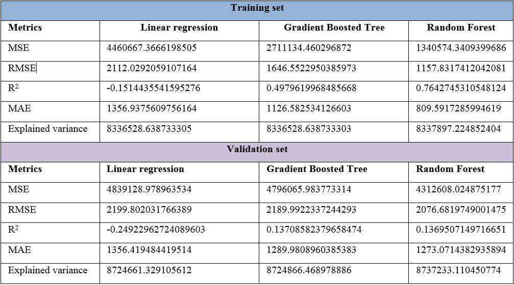
You have already seen that the LR model is much easier to train for a small training dataset. However, we haven't experienced better accuracy compared to GBT and Random Forest models. However, the simplicity of the LR model is a very good starting point. On the other hand, we already argued that Random Forest would be the winner over GBT for several reasons, of course. Let's see the results in a table:
Now let's see how the predictions went for each model for 20 accidents or damage claims:
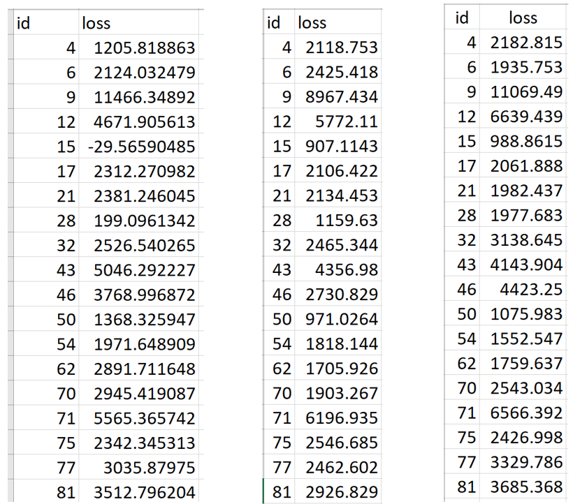
Therefore, based on table 2, it is clear that we should go with the Random Forest regressor to not only predict the insurance claim loss but also its production. Now we will see a quick overview of how to take our best model, that is, an Random Forest regressor into production. The idea is, as a data scientist, you may have produced an ML model and handed it over to an engineering team in your company for deployment in a production-ready environment.
Here, I provide a naïve approach, though IT companies must have their own way to deploy the models. Nevertheless, there will be a dedicated section at the end of this topic. This scenario can easily become a reality by using model persistence—the ability to save and load models that come with Spark. Using Spark, you can either:
- Save and load a single model
- Save and load a full pipeline
A single model is pretty simple, but less effective and mainly works on Spark MLlib-based model persistence. Since we are more interested in saving the best model, that is, the Random Forest regressor model, at first we will fit an Random Forest regressor using Scala, save it, and then load the same model back using Scala:
// Estimator algorithm
val model = new RandomForestRegressor()
                    .setFeaturesCol("features")
                    .setLabelCol("label")
                    .setImpurity("gini")
                    .setMaxBins(20)
                    .setMaxDepth(20)
                    .setNumTrees(50)
fittedModel = rf.fit(trainingData)
We can now simply call the write.overwrite().save() method to save this model to local storage, HDFS, or S3, and the load method to load it right back for future use:
fittedModel.write.overwrite().save("model/RF_model")
val sameModel = CrossValidatorModel.load("model/RF_model")
Now the thing that we need to know is how to use the restored model for making predictions. Here's the answer:
sameModel.transform(Preproessing.testData)
    .select("id", "prediction")
    .withColumnRenamed("prediction", "loss")
    .coalesce(1)
    .write.format("com.databricks.spark.csv")
    .option("header", "true")
    .save("output/result_RF_reuse.csv")
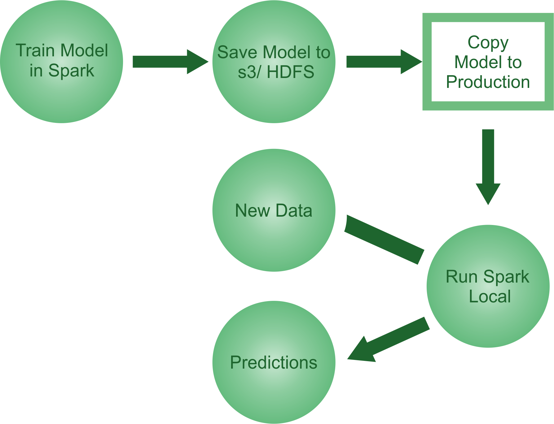
So far, we have only looked at saving and loading a single ML model but not a tuned or stable one. It might even provide you with many wrong predictions. Therefore, now the second approach might be more effective.
The reality is that, in practice, ML workflows consist of many stages, from feature extraction and transformation to model fitting and tuning. Spark ML provides pipelines to help users construct these workflows. Similarly, a pipeline with the cross-validated model can be saved and restored back the same way as we did in the first approach.
We fit the cross-validated model with the training set:
val cvModel = cv.fit(Preproessing.trainingData)
Then we save the workflow/pipeline:
cvModel.write.overwrite().save("model/RF_model")
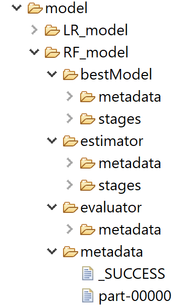
Note that the preceding line of code will save the model in your preferred location with the following directory structure:
//Then we restore the same model back:
val sameCV = CrossValidatorModel.load("model/RF_model")
Now when you try to restore the same model, Spark will automatically pick the best one. Finally, we reuse this model for making a prediction as follows:
sameCV.transform(Preproessing.testData)
      .select("id", "prediction")
      .withColumnRenamed("prediction", "loss")
      .coalesce(1)
      .write.format("com.databricks.spark.csv")
      .option("header", "true")
      .save("output/result_RF_reuse.csv")


