Search icon CANCEL
Subscription
0
Cart icon
Your Cart (0 item)
Close icon
You have no products in your basket yet
Arrow left icon
Explore Products
Best Sellers
New Releases
Books
Videos
Audiobooks
Learning Hub
Conferences
Free Learning
Arrow right icon
Arrow up icon
GO TO TOP
PyTorch 1.x Reinforcement Learning Cookbook

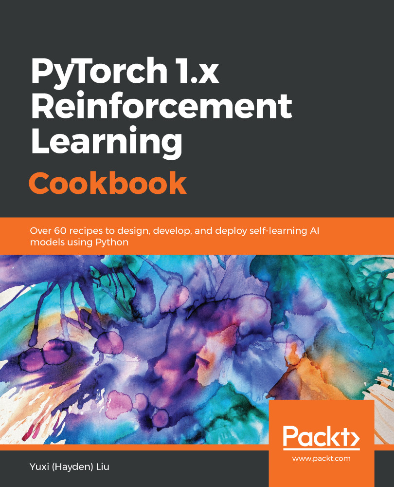
You're reading from   PyTorch 1.x Reinforcement Learning Cookbook Over 60 recipes to design, develop, and deploy self-learning AI models using Python

Arrow left icon
Product type Paperback
Published in Oct 2019
Publisher Packt
ISBN-13 9781838551964
Length 340 pages
Edition 1st Edition
Languages
Tools
Arrow right icon
Author (1):
Arrow left icon
Yuxi (Hayden) Liu Yuxi (Hayden) Liu
Author Profile Icon Yuxi (Hayden) Liu
Yuxi (Hayden) Liu
Arrow right icon
View More author details
Toc

Table of Contents (11) Chapters Close

Preface 1. Getting Started with Reinforcement Learning and PyTorch 2. Markov Decision Processes and Dynamic Programming FREE CHAPTER 3. Monte Carlo Methods for Making Numerical Estimations 4. Temporal Difference and Q-Learning 5. Solving Multi-armed Bandit Problems 6. Scaling Up Learning with Function Approximation 7. Deep Q-Networks in Action 8. Implementing Policy Gradients and Policy Optimization 9. Capstone Project – Playing Flappy Bird with DQN 10. Other Books You May Enjoy

Developing a policy gradient algorithm

The last recipe of the first chapter is about solving the CartPole environment with a policy gradient algorithm. This may be more complicated than we need for this simple problem, in which the random search and hill-climbing algorithms suffice. However, it is a great algorithm to learn, and we will use it in more complicated environments later in the book.

In the policy gradient algorithm, the model weight moves in the direction of the gradient at the end of each episode. We will explain the computation of gradients in the next section. Also, in each step, it samples an action from the policy based on the probabilities computed using the state and weight. It no longer takes an action with certainty, in contrast with random search and hill climbing (by taking the action achieving the higher score). Hence, the policy switches from deterministic to stochastic.

How to do it...

Now, it is time to implement the policy gradient algorithm with PyTorch:

  1. As before, import the necessary packages, create an environment instance, and obtain the dimensions of the observation and action space:
>>> import gym
>>> import torch
>>> env = gym.make('CartPole-v0')
>>> n_state = env.observation_space.shape[0]
>>> n_action = env.action_space.n
  1. We define the run_episode function, which simulates an episode given the input weight and returns the total reward and the gradients computed. More specifically, it does the following tasks in each step:
  • Calculates the probabilities, probs, for both actions based on the current state and input weight
  • Samples an action, action, based on the resulting probabilities
  • Computes the derivatives, d_softmax, of the softmax function with the probabilities as input
  • Divides the resulting derivatives, d_softmax, by the probabilities, probs, to get the derivatives, d_log, of the log term with respect to the policy
  • Applies the chain rule to compute the gradient, grad, of the weights
  • Records the resulting gradient, grad
  • Performs the action, accumulates the reward, and updates the state

Putting all of this into code, we have the following:

 >>> def run_episode(env, weight):
... state = env.reset()
... grads = []
... total_reward = 0
... is_done = False
... while not is_done:
... state = torch.from_numpy(state).float()
... z = torch.matmul(state, weight)
... probs = torch.nn.Softmax()(z)
... action = int(torch.bernoulli(probs[1]).item())
... d_softmax = torch.diag(probs) -
probs.view(-1, 1) * probs
... d_log = d_softmax[action] / probs[action]
... grad = state.view(-1, 1) * d_log
... grads.append(grad)
... state, reward, is_done, _ = env.step(action)
... total_reward += reward
... if is_done:
... break
... return total_reward, grads

After an episode finishes, it returns the total reward obtained in this episode and the gradients computed for the individual steps. These two outputs will be used to update the weight.

  1. Let's make it 1,000 episodes for now:
>>> n_episode = 1000

This means we will run run_episode and n_episodetimes.

  1. Initiate the weight:
>>> weight = torch.rand(n_state, n_action)

We will also record the total reward for every episode:

>>> total_rewards = []
  1. At the end of each episode, we need to update the weight using the computed gradients. For every step of the episode, the weight moves by learning rate * gradient calculated in this step * total reward in the remaining steps. Here, we choose 0.001 as the learning rate:
>>> learning_rate = 0.001

Now, we can run n_episodeepisodes:

 >>> for episode in range(n_episode):
... total_reward, gradients = run_episode(env, weight)
... print('Episode {}: {}'.format(episode + 1, total_reward))
... for i, gradient in enumerate(gradients):
... weight += learning_rate * gradient * (total_reward - i)
... total_rewards.append(total_reward)
……
……
Episode 101: 200.0
Episode 102: 200.0
Episode 103: 200.0
Episode 104: 190.0
Episode 105: 133.0
……
……
Episode 996: 200.0
Episode 997: 200.0
Episode 998: 200.0
Episode 999: 200.0
Episode 1000: 200.0
  1. Now, we calculate the average total reward achieved by the policy gradient algorithm:
 >>> print('Average total reward over {} episode: {}'.format(
n_episode, sum(total_rewards) / n_episode))
Average total reward over 1000 episode: 179.728
  1. We also plot the total reward for every episode as follows:
 >>> import matplotlib.pyplot as plt
>>> plt.plot(total_rewards)
>>> plt.xlabel('Episode')
>>> plt.ylabel('Reward')
>>> plt.show()

In the resulting plot, we can see a clear upward trend before it stays at the maximum value:

We can also see that the rewards oscillate even after it converges. This is because the policy gradient algorithm is a stochastic policy.

  1. Now, let's see how the learned policy performs on 100 new episodes:
 >>> n_episode_eval = 100
>>> total_rewards_eval = []
>>> for episode in range(n_episode_eval):
... total_reward, _ = run_episode(env, weight)
... print('Episode {}: {}'.format(episode+1, total_reward))
... total_rewards_eval.append(total_reward)
...
Episode 1: 200.0
Episode 2: 200.0
Episode 3: 200.0
Episode 4: 200.0
Episode 5: 200.0
……
……
Episode 96: 200.0
Episode 97: 200.0
Episode 98: 200.0
Episode 99: 200.0
Episode 100: 200.0

Let's see the average performance:

>>> print('Average total reward over {} episode: {}'.format(n_episode, sum(total_rewards) / n_episode))
Average total reward over 1000 episode: 199.78

The average reward for the testing episodes is close to the maximum value of 200 for the learned policy. You can re-run the evaluation multiple times. The results are pretty consistent.

How it works...

The policy gradient algorithm trains an agent by taking small steps and updating the weight based on the rewards associated with those steps at the end of an episode. The technique of having the agent run through an entire episode and then updating the policy based on the rewards obtained is called Monte Carlo policy gradient.

The action is selected based on the probability distribution computed based on the current state and the model’s weight. For example, if the probabilities for the left and right actions are [0.6, 0.4], this means the left action is selected 60% of the time; it doesn't mean the left action is chosen, as in the random search and hill-climbing algorithms.

We know that the reward is 1 for each step before an episode terminates. Hence, the future reward we use to calculate the policy gradient at each step is the number of steps remaining. After each episode, we feed the gradient history multiplied by the future rewards to update the weight using the stochastic gradient ascent method. In this way, the longer an episode is, the bigger the update of the weight. This will eventually increase the chance of getting a larger total reward.

As we mentioned at the start of this section, the policy gradient algorithm might be overkill for a simple environment such as CartPole, but it should get us ready for more complicated problems.

There's more...

If we examine the reward/episode plot, it seems that we can also stop early during training when it has been solved – the average reward over 100 consecutive episodes is no less than 195. We just add the following lines of code to the training session:

 >>> if episode >= 99 and sum(total_rewards[-100:]) >= 19500:
... break

Re-run the training session. You should get something similar to the following, which stops after several hundred episodes:

Episode 1: 10.0
Episode 2: 27.0
Episode 3: 28.0
Episode 4: 15.0
Episode 5: 12.0
……
……
Episode 549: 200.0
Episode 550: 200.0
Episode 551: 200.0
Episode 552: 200.0
Episode 553: 200.0

See also

lock icon The rest of the chapter is locked
Register for a free Packt account to unlock a world of extra content!
A free Packt account unlocks extra newsletters, articles, discounted offers, and much more. Start advancing your knowledge today.
Unlock this book and the full library FREE for 7 days
Get unlimited access to 7000+ expert-authored eBooks and videos courses covering every tech area you can think of
Renews at $19.99/month. Cancel anytime
Banner background image