Let's begin by importing the necessary libraries:
- Import the required Python libraries and a linear regression class:
import pandas as pd
import numpy as np
import matplotlib.pyplot as plt
import seaborn as sns
from sklearn.linear_model import LinearRegression
To proceed with this recipe, let's create a toy dataframe with an x variable that follows a normal distribution and shows a linear relationship with a y variable.
- Create an x variable with 200 observations that are normally distributed:
np.random.seed(29)
x = np.random.randn(200)
Setting the seed for reproducibility using np.random.seed() will help you get the outputs shown in this recipe.
- Create a y variable that is linearly related to x with some added random noise:
y = x * 10 + np.random.randn(200) * 2
- Create a dataframe with the x and y variables:
data = pd.DataFrame([x, y]).T
data.columns = ['x', 'y']
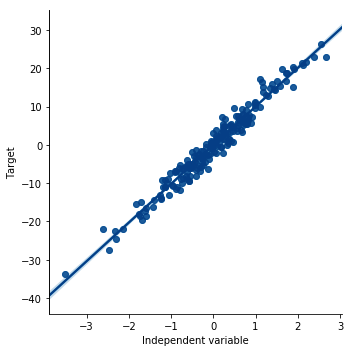
- Plot a scatter plot to visualize the linear relationship:
sns.lmplot(x="x", y="y", data=data, order=1)
plt.ylabel('Target')
plt.xlabel('Independent variable')
The preceding code results in the following output:

To evaluate the linear relationship using residual plots, we need to carry out a few more steps.
- Build a linear regression model between x and y:
linreg = LinearRegression()
linreg.fit(data['x'].to_frame(), data['y'])
Scikit-learn predictor classes do not take pandas Series as arguments. Because data['x'] is a pandas Series, we need to convert it into a dataframe using to_frame().
Now, we need to calculate the residuals.
- Make predictions of y using the fitted linear model:
predictions = linreg.predict(data['x'].to_frame())
- Calculate the residuals, that is, the difference between the predictions and the real outcome, y:
residuals = data['y'] - predictions
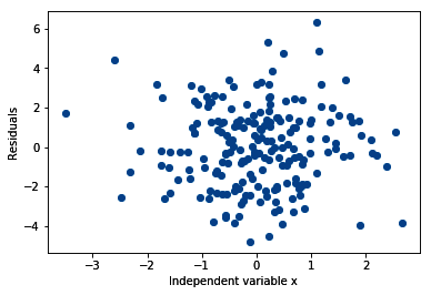
- Make a scatter plot of the independent variable x and the residuals:
plt.scatter(y=residuals, x=data['x'])
plt.ylabel('Residuals')
plt.xlabel('Independent variable x')
The output of the preceding code is as follows:

- Finally, let's evaluate the distribution of the residuals:
sns.distplot(residuals, bins=30)
plt.xlabel('Residuals')
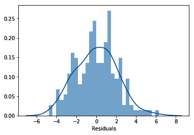
In the following output, we can see that the residuals are normally distributed and centered around zero:
