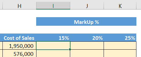
The following example, which is using the same Sales Report worksheet, seeks to compare sales that are obtained by using MarkUps of 15%, 20%, and 25%.
In this case, the sales is calculated as Cost of Sales × (1+MarkUp %). This is a screenshot of the layout for the markup:

Mixed referencing is required when you need to lock a reference in one direction only, either down or across to the right, but not both. In the following example, you will create the formula in cell I5, and then copy it down through rows 6 to 20 and across columns J and K. The following screenshot shows the calculation of 15% MarkUp:

The base formula is H5*(1+I4).
Note that there are two cell references in the formula, H5 and I4, which you will need to consider individually.
Cell H5 is the Cost of Sales. The column part is H, which we will look at when we consider copying to the right...


