Search icon CANCEL
Subscription
0
Cart icon
Your Cart (0 item)
Close icon
You have no products in your basket yet
Arrow left icon
Explore Products
Best Sellers
New Releases
Books
Videos
Audiobooks
Learning Hub
Conferences
Free Learning
Arrow right icon
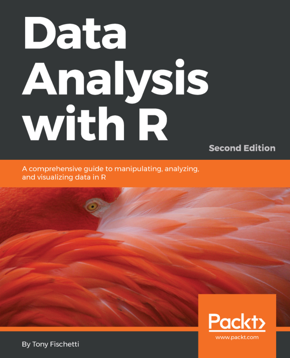
Data Analysis with R, Second Edition

Data Analysis with R, Second Edition: A comprehensive guide to manipulating, analyzing, and visualizing data in R , Second Edition

eBook
€8.99 €26.99
Paperback
€32.99
Subscription
Free Trial
Renews at €18.99p/m

What do you get with eBook?

Product feature icon Instant access to your Digital eBook purchase
Product feature icon Download this book in EPUB and PDF formats
Product feature icon Access this title in our online reader with advanced features
Product feature icon DRM FREE - Read whenever, wherever and however you want
OR
Modal Close icon
Payment Processing...
tick Completed

Billing Address

Table of content icon View table of contents Preview book icon Preview Book

Data Analysis with R, Second Edition

RefresheR

Before we dive into the (other) fun stuff (sampling multi-dimensional probability distributions, using convex optimization to fit data models, and so on), it would be helpful if we review those aspects of R that all subsequent chapters will assume knowledge of.

If you fancy yourself an R guru, you should still, at least, skim through this chapter, because you'll almost certainly find the idioms, packages, and style introduced here to be beneficial for following the rest of the material.

If you don't care much about R (yet), and are just in this for the statistics, you can heave a heavy sigh of relief that, for the most part, you can run the code given in this book in the interactive R interpreter with very little modification and just follow along with the ideas. However, it is my belief (read: delusion) that by the end of this book, you'll cultivate a newfound appreciation for R alongside a robust understanding of methods in data analysis.

Fire up your R interpreter and let's get started!

Navigating the basics

In the interactive R interpreter, any line starting with a > character denotes R asking for input. (If you see a + prompt, it means that you didn't finish typing a statement at the prompt and R is asking you to provide the rest of the expression). Striking the return key will send your input to R to be evaluated. R's response is then spit back at you in the line immediately following your input, after which R asks for more input. This is called a REPL (Read-Evaluate-Print-Loop). It is also possible for R to read a batch of commands saved in a file (unsurprisingly called batch mode), but we'll be using the interactive mode for most of the book.

As you might imagine, R supports all the familiar mathematical operators as with most other languages.

Arithmetic and assignment

Check out the following example:

  > 2 + 2 
  [1] 4 
 
  > 9 / 3 
  [1] 3 
 
  > 5 %% 2    # modulus operator (remainder of 5 divided by 2) 
  [1] 1 

Anything that occurs after the octothorpe or pound sign, #, (or hash-tag for you young'uns), is ignored by the R interpreter. This is useful to document the code in natural language. These are called comments.

In a multi-operation arithmetic expression, R will follow the standard order of operations from math. In order to override this natural order, you have to use parentheses flanking the sub-expression that you'd like to be performed first:

   > 3 + 2 - 10 ^ 2        # ^ is the exponent operator 
   [1] -95 
   > 3 + (2 - 10) ^ 2 
   [1] 67 

In practice, almost all compound expressions are split up with intermediate values assigned to variables that, when used in future expressions, are just like substituting the variable with the value that was assigned to it. The (primary) assignment operator is <-:

   > # assignments follow the form VARIABLE <- VALUE 
   > var <- 10 
   > var 
   [1] 10 
   > var ^ 2 
   [1] 100 
   > VAR / 2             # variable names are case-sensitive  
   Error: object 'VAR' not found 

Notice that the first and second lines in the preceding code snippet didn't have an output to be displayed, so R just immediately asked for more input. This is because assignments don't have a return value. Their only job is to give a value to a variable or change the existing value of a variable. Generally, operations and functions on variables in R don't change the value of the variable. Instead, they return the result of the operation. If you want to change a variable to the result of an operation using that variable, you have to reassign that variable as follows:

   > var               # var is 10 
   [1] 10 
   > var ^ 2 
   [1] 100 
   > var               # var is still 10 
   [1] 10 
   > var <- var ^ 2    # no return value 
   > var               # var is now 100 
   [1] 100 

Be aware that variable names may contain numbers, underscores, and periods; this is something that trips up a lot of people who are familiar with other programming languages that disallow using periods in variable names. The only further restrictions on variable names are that they must start with a letter (or a period and then a letter), and that it must not be one of the reserved words in R such as TRUE, Inf, and so on.

Although the arithmetic operators that we've seen thus far are functions in their own right, most functions in R take the form,  function_name(value(s) supplied to the function). The values supplied to the function are called arguments of that function:

   > cos(3.14159)      # cosine function 
   [1] -1 
   > cos(pi)           # pi is a constant that R provides 
   [1] -1 
   > acos(-1)          # arccosine function 
   [1] 3.141593
   > acos(cos(pi)) + 10  
   [1] 13.14159 
   > # functions can be used as arguments to other functions 

If you paid attention in math class, you'll know that the cosine of pi is -1 and that arccosine is the inverse function of cosine.

There are hundreds of such useful functions defined in base R, only a handful of which we will see in this book. Two sections from now, we will be building our very own functions.

Before we move on from arithmetic, it will serve us well to visit some of the odd values that may result from certain operations:

   > 1 / 0 
   [1] Inf 
   > 0 / 0 
   [1] NaN 

It is common during practical usage of R to accidentally divide by zero. As you can see, this undefined operation yields an infinite value in R. Dividing zero by zero yields the value NaN, which stands for Not a Number.

Logicals and characters

So far, we've only been dealing with numerics, but there are other atomic data types in R:

   > foo <- TRUE        # foo is of the logical data type 
   > class(foo)         # class() tells us the type 
   [1] "logical" 
   > bar <- "hi!"       # bar is of the character data type 
   > class(bar) 
   [1] "character" 

The logical data type (also called Booleans) can hold the values TRUE or FALSE or, equivalently, T or F. The familiar operators from Boolean algebra are defined for these types:

   > foo 
   [1] TRUE 
   > foo && TRUE                 # boolean and 
   [1] TRUE 
   > foo && FALSE 
   [1] FALSE 
   > foo || FALSE                # boolean or 
   [1] TRUE 
   > !foo                        # negation operator 
   [1] FALSE 

In a Boolean expression with a logical value and a number, any number that is not 0 is interpreted as TRUE:

   > foo && 1 
   [1] TRUE 
   > foo && 2 
   [1] TRUE 
   > foo && 0 
   [1] FALSE 

Additionally, there are functions and operators that return logical values such as the following:

   > 4 < 2           # less than operator 
   [1] FALSE 
   > 4 >= 4          # greater than or equal to 
   [1] TRUE 
   > 3 == 3          # equality operator 
   [1] TRUE 
   > 3 != 2          # inequality operator 
   [1] TRUE 

Just as there are functions in R that are only defined for work on the numeric and logical data type, there are other functions that are designed to work only with the character data type, also known as strings:

   > lang.domain <- "statistics" 
   > lang.domain <- toupper(lang.domain) 
   > print(lang.domain) 
   [1] "STATISTICS" 
   > # retrieves substring from first character to fourth character 
   > substr(lang.domain, 1, 4)           
   [1] "STAT" 
   > gsub("I", "1", lang.domain)  # substitutes every "I" for "1" 
   [1] "STAT1ST1CS" 
   > # combines character strings 
   > paste("R does", lang.domain, "!!!") 
   [1] "R does STATISTICS !!!" 

Flow of control

The last topic in this section will be flow of control constructs.

The most basic flow of control construct is the if statement. The argument to an if statement (what goes between the parentheses) is an expression that returns a logical value. The block of code following the if statement gets executed only if the expression yields TRUE:

   > if(2 + 2 == 4) 
   +   print("very good") 
  [1] "very good" 
   > if(2 + 2 == 5) 
   +    print("all hail to the thief") 

It is possible to execute more than one statement if an if condition is triggered; you just have to use curly brackets ({}) to contain the statements:

   > if((4/2==2) && (2*2==4)){ 
   +    print("four divided by two is two...") 
   +    print("and two times two is four") 
   + } 
  [1] "four divided by two is two..." 
  [1] "and two times two is four"  

It is also possible to specify a block of code that will get executed if the if conditional is FALSE:

   > closing.time <- TRUE 
   > if(closing.time){ 
   +    print("you don't have to go home") 
   +    print("but you can't stay here") 
   + } else{ 
   +    print("you can stay here!") 
   + } 
  [1] "you don't have to go home" 
  [1] "but you can't stay here" 
  > if(!closing.time){ 
  +     print("you don't have to go home") 
  +     print("but you can't stay here") 
  + } else{ 
  +     print("you can stay here!") 
  + } 
  [1] "you can stay here!"  

There are other flow of control constructs (like while and for), but we won't be directly using them much in this text.

Getting help in R

Before we go further, it would serve us well to have a brief section detailing how to get help in R. Most R tutorials leave this for one of the last sections--if it is even included at all! In my own personal experience, though, getting help is going to be one of the first things you will want to do as you add more bricks to your R knowledge castle. Learning R doesn't have to be difficult; just take it slowly, ask questions, and get help early. Go you!

It is easy to get help with R right at the console. Running the help.start() function at the prompt will start a manual browser. From here, you can do anything from going over the basics of R to reading the nitty-gritty details on how R works internally.

You can get help with a particular function in R if you know its name, by supplying that name as an argument to the help function. For example, let's say you want to know more about the gsub() function that I sprang on you before. Check out the following code:

  > help("gsub") 
  > # or simply 
  > ?gsub 

This will display a manual page documenting what the function is, how to use it, and examples of its usage.

This rapid accessibility to documentation means that I'm never hopelessly lost when I encounter a function that I haven't seen before. The downside to this extraordinarily convenient help mechanism is that I rarely bother to remember the order of arguments as looking them up is just seconds away.

Occasionally, you won't quite remember the exact name of the function that you're looking for, but you'll have an idea about what the name should be. For this, you can use the help.search() function:

   > help.search("chisquare") 
   > # or simply 
   > ??chisquare 

For tougher, more semantic queries, nothing beats a good old fashioned web search engine. If you don't get relevant results the first time, try adding the term programming or statistics in there for good measure.

Vectors

Vectors are the most basic data structures in R, and they are ubiquitous indeed. In fact, even the single values that we've been working with thus far were actually vectors of length 1. That's why the interactive R console has been printing [1] along with all of our output.

Vectors are essentially an ordered collection of values of the same atomic data type. Vectors can be arbitrarily large (with some limitations) or they can be just one single value.

The canonical way of building vectors manually is using the c() function (which stands for combine):

  > our.vect <- c(8, 6, 7, 5, 3, 0, 9) 
  > our.vect 
  [1] 8 6 7 5 3 0 9 

In the preceding example, we created a numeric vector of length 7 (namely, Jenny's telephone number).

Let's try to put character data types into this vector as follows:

  > another.vect <- c("8", 6, 7, "-", 3, "0", 9) 
  > another.vect 
  [1] "8" "6" "7" "-" "3" "0" "9" 

R would convert all the items in the vector (called elements) into character data types to satisfy the condition that all elements of a vector must be of the same type. A similar thing happens when you try to use logical values in a vector with numbers; the logical values would be converted into 1 and 0 (for TRUE and FALSE, respectively). These logicals will turn into TRUE and FALSE (note the quotation marks) when used in a vector that contains characters.

Subsetting

It is very common to want to extract one or more elements from a vector. For this, we use a technique called indexing or subsetting. After the vector, we put an integer in square brackets ([]) called the subscript operator. This instructs R to return the element at that index. The indices (plural for index, in case you were wondering!) for vectors in R start at 1 and stop at the length of the vector:

  > our.vect[1]                  # to get the first value 
  [1] 8 
  > # the function length() returns the length of a vector 
  > length(our.vect) 
  [1] 7 
  > our.vect[length(our.vect)]   # get the last element of a vector 
  [1] 9 

Note that in the preceding code, we used a function in the subscript operator. In cases like these, R evaluates the expression in the subscript operator and uses the number it returns as the index to extract.

If we get greedy and try to extract an element from an index that doesn't exist, R will respond with NA, meaning, not available. We see this special value cropping up from time to time throughout this text:

  > our.vect[10] 
  [1] NA 

One of the most powerful ideas in R is that you can use vectors to subset other vectors:

  > # extract the first, third, fifth, and 
  > # seventh element from our vector 
  > our.vect[c(1, 3, 5, 7)] 
  [1] 8 7 3 9 

The ability to use vectors to index other vectors may not seem like much now, but its usefulness will become clear soon.

Another way to create vectors is using sequences:

  > other.vector <- 1:10 
  > other.vector 
  [1]  1  2  3  4  5  6  7  8  9 10 
  > another.vector <- seq(50, 30, by=-2) 
  > another.vector 
  [1] 50 48 46 44 42 40 38 36 34 32 30 

Here, the 1:10 statement creates a vector from 1 to 10. 10:1 would have created the same 10-element vector, but in reverse. The seq() function is more general in that it allows sequences to be made using steps (among many other things).

Combining our knowledge of sequences and vectors subsetting vectors, we can get the first five digits of Jenny's number:

  > our.vect[1:5] 
  [1] 8 6 7 5 3 

Vectorized functions

Part of what makes R so powerful is that many of R's functions take vectors as arguments. These vectorized functions are usually extremely fast and efficient. We've already seen one such function, length(), but there are many, many others:

  > # takes the mean of a vector 
  > mean(our.vect) 
  [1] 5.428571 
  > sd(our.vect)    # standard deviation 
  [1] 3.101459 
  > min(our.vect) 
  [1] 0 
  > max(1:10) 
  [1] 10 
  > sum(c(1, 2, 3)) 
  [1] 6 

In practical settings, such as when reading data from files, it is common to have NA values in vectors:

  > messy.vector <- c(8, 6, NA, 7, 5, NA, 3, 0, 9) 
  > messy.vector 
  [1]  8  6 NA  7  5 NA  3  0  9 
  > length(messy.vector) 
  [1] 9 

Some vectorized functions will not allow NA values by default. In these cases, an extra keyword argument must be supplied along with the first argument to the function:

  > mean(messy.vector) 
  [1] NA 
  > mean(messy.vector, na.rm=TRUE) 
  [1] 5.428571 
  > sum(messy.vector, na.rm=FALSE) 
  [1] NA 
  > sum(messy.vector, na.rm=TRUE) 
  [1] 38 

As mentioned previously, vectors can be constructed from logical values as well:

  > log.vector <- c(TRUE, TRUE, FALSE) 
  > log.vector 
  [1]  TRUE TRUE FALSE 

Since logical values can be coerced into behaving like numerics, as we saw earlier, if we try to sum a logical vector as follows:

  > sum(log.vector) 
  [1] 2 

We will, essentially, get a count of the number of TRUE values in that vector.

There are many functions in R that operate on vectors and return logical vectors. is.na() is one such function. It returns a logical vector, that is, the same length as the vector supplied as an argument, with a TRUE in the position of every NA value. Remember our messy vector (from just a minute ago)?

  > messy.vector 
  [1]  8  6 NA  7  5 NA  3  0  9 
  > is.na(messy.vector) 
  [1] FALSE FALSE  TRUE FALSE FALSE  TRUE FALSE FALSE FALSE 
  > #  8     6      NA   7     5      NA   3       0    9 

Putting together these pieces of information, we can get a count of the number of NA values in a vector as follows:

  > sum(is.na(messy.vector)) 
  [1] 2 

When you use Boolean operators on vectors, they also return logical vectors of the same length as the vector being operated on:

  > our.vect > 5 
  [1]  TRUE  TRUE  TRUE FALSE FALSE FALSE  TRUE 

If we wanted to--and we do--count the number of digits in Jenny's phone number that are greater than five, we would do so in the following manner:

  > sum(our.vect > 5) 
  [1] 4 

Advanced subsetting

Did I mention that we can use vectors to subset other vectors! When we subset vectors using logical vectors of the same length, only the elements corresponding to the TRUE values are extracted. Hopefully, light bulbs are starting to go off in your head. If we wanted to extract only the legitimate non-NA digits from Jenny's number, we can do it as follows:

  > messy.vector[!is.na(messy.vector)] 
  [1] 8 6 7 5 3 0 9 

This is a very critical trait of R, so let's take our time understanding it; this idiom will come up again and again throughout this book.

The logical vector that yields TRUE when an NA value occurs in messy.vector (from is.na()) is then negated (the whole thing) by the negation operator,  !. The resultant vector is TRUE whenever the corresponding value in messy.vector is not NA. When this logical vector is used to subset the original messy vector, it only extracts the non-NA values from it.

Similarly, we can show all the digits in Jenny's phone number that are greater than five as follows:

  > our.vect[our.vect > 5] 
  [1] 8 6 7 9 

Thus far, we've only been displaying elements that have been extracted from a vector. However, just as we've been assigning and reassigning variables, we can assign values to various indices of a vector and change the vector as a result. For example, if Jenny tells us that we have the first digit of her phone number wrong (it's really 9), we can reassign just that element without modifying the others:

  > our.vect 
  [1] 8 6 7 5 3 0 9 
  > our.vect[1] <- 9 
  > our.vect 
  [1] 9 6 7 5 3 0 9 

Sometimes, it may be required to replace all the NA values in a vector with the value 0. To do this with our messy vector, we can execute the following command:

  > messy.vector[is.na(messy.vector)] <- 0 
  > messy.vector 
  [1] 8 6 0 7 5 0 3 0 9 

Elegant though the preceding solution is, modifying a vector in place is usually discouraged in favor of creating a copy of the original vector and modifying the copy. One such technique to perform this is using the ifelse() function.

Not to be confused with the if/else control construct, ifelse() is a function that takes three arguments: a test that returns a logical/Boolean value, a value to use if the element passes the test, and one to return if the element fails the test.

The preceding in-place modification solution could be reimplemented with ifelse as follows:

  > ifelse(is.na(messy.vector), 0, messy.vector) 
  [1] 8 6 0 7 5 0 3 0 9 

Recycling

The last important property of vectors and vector operations in R is that they can be recycled. To understand what I mean, examine the following expression:

  > our.vect + 3 
  [1] 12  9 10  8  6  3 12 

This expression adds three to each digit in Jenny's phone number. Although it may look so, R is not performing this operation between a vector and a single value. Remember when I said that single values are actually vectors of the length 1? What is really happening here is that R is told to perform element-wise addition on a vector of length 7 and a vector of length 1. As element-wise addition is not defined for vectors of differing lengths, R recycles the smaller vector until it reaches the same length as that of the bigger vector. Once both the vectors are the same size, then R, element by element, performs the addition and returns the result:

  > our.vect + 3 
  [1] 12  9 10  8  6  3 12 

This is tantamount to the following:

  > our.vect + c(3, 3, 3, 3, 3, 3, 3) 
  [1] 12  9 10  8  6  3 12 

If we wanted to extract every other digit from Jenny's phone number, we can do so in the following manner:

  > our.vect[c(TRUE, FALSE)] 
  [1] 9 7 3 9 

This works because the vector c(TRUE, FALSE) is repeated until it is of the length 7, making it equivalent to the following:

  > our.vect[c(TRUE, FALSE, TRUE, FALSE, TRUE, FALSE, TRUE)] 
  [1] 9 7 3 9 

One common snag related to vector recycling that R users (useRs, if I may) encounter is that during some arithmetic operations involving vectors of discrepant length, R will warn you if the smaller vector cannot be repeated a whole number of times to reach the length of the bigger vector. This is not a problem when doing vector arithmetic with single values as 1 can be repeated any number of times to match the length of any vector (which must, of course, be an integer). It would pose a problem, though, if we were looking to add three to every other element in Jenny's phone number:

  > our.vect + c(3, 0) 
  [1] 12  6 10  5  6  0 12 
  Warning message: 
  In our.vect + c(3, 0) : 
    longer object length is not a multiple of shorter object length 

You will likely learn to love these warnings as they have stopped many useRs from making grave errors.

Before we move on to the next section, an important thing to note is that in a lot of other programming languages, many of the things that we did would have been implemented using for loops and other control structures. Although there is certainly a place for loops and such in R, often a more sophisticated solution exists in using just vector/matrix operations. In addition to elegance and brevity, the solution that exploits vectorization and recycling is often much more efficient.

Functions

If we need to perform some computation that isn't already a function in R a multiple number of times, we usually do so by defining our own functions. A custom function in R is defined using the following syntax:

  > function.name <- function(argument1, argument2, ...){ 
  +   # some functionality 
  + } 

For example, if we wanted to write a function that determined if a number supplied as an argument was even, we can do so in the following manner:

  > is.even <- function(a.number){ 
  +   remainder <- a.number %% 2 
  +   if(remainder==0) 
  +     return(TRUE) 
  +   return(FALSE) 
  + } 
   
  > # testing it 
  > is.even(10) 
  [1] TRUE 
  > is.even(9) 
  [1] FALSE 

As an example of a function that takes more than one argument, let's generalize the preceding function by creating a function that determines whether the first argument is divisible by its second argument:

  > is.divisible.by <- function(large.number, smaller.number){ 
  +   if(large.number %% smaller.number != 0) 
  +     return(FALSE) 
  +   return(TRUE) 
  + } 
   
  > # testing it 
  > is.divisible.by(10, 2) 
  [1] TRUE 
  > is.divisible.by(10, 3) 
  [1] FALSE 
  > is.divisible.by(9, 3) 
  [1] TRUE 

Our function, is.even(), could now be rewritten simply as follows:

  > is.even <- function(num){ 
  +   is.divisible.by(num, 2) 
  + } 

It is very common in R to want to apply a particular function to every element of a vector. Instead of using a loop to iterate over the elements of a vector, as we would do in many other languages, we use a function called sapply() to perform this. sapply() takes a vector and a function as its arguments. It then applies the function to every element and returns a vector of results. We can use sapply() in this manner to find out which digits in Jenny's phone number are even:

  > sapply(our.vect, is.even) 
  [1] FALSE  TRUE FALSE FALSE FALSE  TRUE FALSE 

This worked great because sapply takes each element and uses it as the argument in is.even(), which takes only one argument. If you wanted to find the digits that are divisible by three, it would require a little bit more work.

One option is just to define a function,  is.divisible.by.three(), that takes only one argument and use this in sapply. The more common solution, however, is to define an unnamed function that does just that in the body of the sapply function call:

  > sapply(our.vect, function(num){is.divisible.by(num, 3)}) 
  [1]  TRUE  TRUE FALSE FALSE  TRUE  TRUE  TRUE 

Here, we essentially created a function that checks whether its argument is divisible by three, except we don't assign it to a variable and use it directly in the sapply body instead. These one-time-use unnamed functions are called anonymous functions or lambda functions. (The name comes from Alonzo Church's invention of the lambda calculus, if you were wondering.)

This is somewhat of an advanced usage of R, but it is very useful as it comes up very often in practice.

If we wanted to extract the digits in Jenny's phone number that are divisible by both, two and three, we can write it as follows:

  > where.even <- sapply(our.vect, is.even) 
  > where.div.3 <- sapply(our.vect, function(num){ 
  +   is.divisible.by(num, 3)}) 
  > # "&" is like the "&&" and operator but for vectors  
  > our.vect[where.even & where.div.3] 
  [1] 6 0 

Neat-O!

Note that if we wanted to be sticklers, we would have a clause in the function bodies to preclude a modulus computation, where the first number was smaller than the second. If we had, our function would not have erroneously indicated that 0 was divisible by two and three. I'm not a stickler, though, so the function will remain as is. Fixing this function is left as an exercise for the (stickler) reader.

Matrices

In addition to the vector data structure, R has the matrix, data frame, list, and array data structures. Though we will be using all of these types (except arrays) in this book, we only need to review the first two in this chapter.

A matrix in R, like in math, is a rectangular array of values (of one type) arranged in rows and columns and can be manipulated as a whole. Operations on matrices are fundamental to data analysis.

One way of creating a matrix is to just supply a vector to the matrix() function:

 > a.matrix <- matrix(c(1, 2, 3, 4, 5, 6)) 
 > a.matrix 
       [,1] 
  [1,]    1  
  [2,]    2  
  [3,]    3  
  [4,]    4  
  [5,]    5  
  [6,]    6 

This produces a matrix with all the supplied values in a single column. We can make a similar matrix with two columns by supplying matrix() with an optional argument, ncol, that specifies the number of columns:

 > a.matrix <- matrix(c(1, 2, 3, 4, 5, 6), ncol=2) 
 > a.matrix 
       [,1] [,2] 
  [1,]    1    4 
  [2,]    2    5 
  [3,]    3    6 

We could have produced the same matrix by binding two vectors, c(1, 2, 3) and c(4, 5, 6), by columns using the cbind() function as follows:

 > a2.matrix <- cbind(c(1, 2, 3), c(4, 5, 6)) 

We could create the transposition of this matrix (where rows and columns are switched) by binding these vectors by row instead:

 > a3.matrix <- rbind(c(1, 2, 3), c(4, 5, 6)) 
 > a3.matrix 
       [,1] [,2] [,3] 
  [1,]    1    2    3 
  [2,]    4    5    6 

We can do this by just using the matrix transposition function in R, t():

 > t(a2.matrix) 

Some other functions that operate on whole vectors are rowSums()/colSums() and rowMeans()/colMeans():

 > a2.matrix 
       [,1] [,2] 
  [1,]    1    4 
  [2,]    2    5 
  [3,]    3    6 
 > colSums(a2.matrix) 
  [1]  6 15 
 > rowMeans(a2.matrix) 
  [1] 2.5 3.5 4.5 

If vectors have sapply(), then matrices have apply(). The preceding two functions could have been written, more verbosely, as follows:

  > apply(a2.matrix, 2, sum) 
  [1]  6 15 
  > apply(a2.matrix, 1, mean) 
  [1] 2.5 3.5 4.5 

Here, 1 instructs R to perform the supplied function over its rows, and 2, over its columns.

The matrix multiplication operator in R is %*%:

  > a2.matrix %*% a2.matrix 
  Error in a2.matrix %*% a2.matrix : non-conformable arguments 

Remember, matrix multiplication is only defined for matrices where the number of columns in the first matrix is equal to the number of rows in the second:

  > a2.matrix 
       [,1] [,2] 
  [1,]    1    4 
  [2,]    2    5 
  [3,]    3    6 
  > a3.matrix 
       [,1] [,2] [,3] 
  [1,]    1    2    3 
  [2,]    4    5    6 
  > a2.matrix %*% a3.matrix 
       [,1] [,2] [,3] 
  [1,]   17   22   27 
  [2,]   22   29   36 
  [3,]   27   36   45 
  > # dim() tells us how many rows and columns 
  > # (respectively) there are in the given matrix 
  > dim(a2.matrix) 
  [1] 3 2 

To index the element of a matrix at the second row and first column, you need to supply both of these numbers into the subscripting operator:

  > a2.matrix[2,1] 
  [1] 2 

Many useRs get confused and forget the order in which the indices must appear; remember, it's row first, then columns!

If you leave one of the spaces empty, R will assume that you want that whole dimension:

  > # returns the whole second column 
  a2.matrix[,2] 
  [1] 4 5 6 
  > # returns the first row 
  > a2.matrix[1,] 
  [1] 1 4 

As always, we can use vectors in our subscript operator:

  > # give me element in column 2 at the first and third row 
  > a2.matrix[c(1, 3), 2] 
  [1] 4 6

Loading data into R

Thus far, we've only been entering data directly into the interactive R console. For any dataset of non-trivial size, this is, obviously, an intractable solution. Fortunately for us, R has a robust suite of functions to read data directly from external files.

Go ahead and create a file on your hard disk called favorites.txt that looks like this:

flavor,number 
pistachio,6 
mint chocolate chip,7 
vanilla,5
chocolate,10 
strawberry,2 
neopolitan,4 

This data represents the number of students in a class that prefer a particular flavor of soy ice cream. We can read the file into a variable called favs as follows:

 > favs <- read.table("favorites.txt", sep=",", header=TRUE) 

If you get an error that there is no such file or directory, give R the full path name to your dataset or, alternatively, run the following command:

 > favs <- read.table(file.choose(), sep=",", header=TRUE) 

The preceding command brings up an open file dialog to let you navigate to the file that you've just created.

The sep="," argument tells R that each data element in a row is separated by a comma. Other common data formats have values separated by tabs and pipes ("|"). The value of sep should then be "\t" and "|", respectively.

The header=TRUE argument tells R that the first row of the file should be interpreted as the names of the columns. Remember, you can enter ?read.table at the console to learn more about these options.

Reading from files in this comma-separated values format (usually with the .csv file extension) is so common that R has a more specific function just for it. The preceding data import expression can be best written simply as follows:

 > favs <- read.csv("favorites.txt") 

Now, we have all the data in the file held in a variable of the data.frame class. A data frame can be thought of as a rectangular array of data that you might see in a spreadsheet application. In this way, a data frame can also be thought of as a matrix; indeed, we can use matrix-style indexing to extract elements from it. A data frame differs from a matrix, though, in that a data frame may have columns of differing types. For example, whereas a matrix would only allow one of these types, the dataset that we just loaded contains character data in its first column and numeric data in its second column.

Let's check out what we have using the head() command, which will show us the first few lines of a data frame:

  > head(favs) 
                 flavor number 
  1           pistachio      6 
  2 mint chocolate chip      7 
  3             vanilla      5 
  4           chocolate     10 
  5          strawberry      2 
  6          neopolitan      4 
 
  > class(favs) 
  [1] "data.frame" 
  > class(favs$flavor) 
  [1] "factor" 
  > class(favs$number) 
  [1] "numeric" 

I lied, okay! So what?! Technically, flavor is a factor data type, not a character type.

We haven't seen factors yet, but the idea behind them is really simple. Essentially, factors are codings for categorical variables, which are variables that take on one of a finite number of categories--think {"high", "medium", and "low"} or {"control", "experimental"}.

Though factors are extremely useful in statistical modeling in R, the fact that R, by default, automatically interprets a column from the data read from disk as a type factor if it contains characters is something that trips up novices and seasoned useRs alike. Due to this, we will primarily prevent this behavior manually by adding the stringsAsFactors optional keyword argument to the read.* commands:

  > favs <- read.csv("favorites.txt", stringsAsFactors=FALSE) 
  > class(favs$flavor) 
  [1] "character" 

Much better, for now! If you'd like to make this behavior the new default, read the ?options manual page. We can always convert to factors later on if we need to!

If you haven't noticed already, I've snuck a new operator on you--$, the extract operator. This is the most popular way to extract attributes (or columns) from a data frame. You can also use double square brackets ([[ and ]]) to do this.

These are both in addition to the canonical matrix indexing option. The following three statements are thus, in this context, functionally identical:

  > favs$flavor 
  [1] "pistachio"           "mint chocolate chip" "vanilla"             
  [4] "chocolate"           "strawberry"          "neopolitan"          
  > favs[["flavor"]] 
  [1] "pistachio"           "mint chocolate chip" "vanilla"             
  [4] "chocolate"           "strawberry"          "neopolitan"          
  > favs[,1] 
  [1] "pistachio"           "mint chocolate chip" "vanilla"             
  [4] "chocolate"           "strawberry"          "neopolitan"   
Notice how R has now printed another number in square brackets--besides [1]--along with our output. This is to show us that chocolate is the fourth element of the vector that was returned from the extraction.

You can use the names() function to get a list of the columns available in a data frame. You can even reassign names using the same:

  > names(favs) 
  [1] "flavor" "number" 
  > names(favs)[1] <- "flav" 
  > names(favs) 
  [1] "flav"   "number" 

Lastly, we can get a compact display of the structure of a data frame using the str() function on it:

  > str(favs) 
  'data.frame': 6 obs. of  2 variables: 
   $ flav  : chr  "pistachio" "mint chocolate chip" "vanilla"   
"chocolate" ...
$ number: num 6 7 5 10 2 4

Actually, you can use this function on any R structure--the property of functions that change their behavior based on the type of input is called polymorphism.

Working with packages

Robust, performant, and numerous though base R functions are, we are by no means limited to them! Additional functionality is available in the form of packages. In fact, what makes R such a formidable statistics platform is the astonishing wealth of packages available (over 10,000 at the time of writing). R's ecosystem is second to none!

Most of these myriad packages exist on the Comprehensive R Archive Network (CRAN). CRAN is the primary repository for user-created packages.

One package that we are going to start using right away is the ggplot2 package. ggplot2 is a plotting system for R. Base R has sophisticated and advanced mechanisms to plot data, but many find ggplot2 more consistent and easier to use. Further, the plots are often more aesthetically pleasing by default.

Let's install it:

  > # downloads and installs from CRAN 
  > install.packages("ggplot2") 

Now that we have the package downloaded, let's load it into the R session and test it out by plotting our data from the last section:

  > library(ggplot2) 
  > ggplot(favs, aes(x=flav, y=number)) + 
  +    geom_bar(stat="identity") + 
  +    ggtitle("Soy ice cream flavor preferences") 

The graph generated by the preceding code will be as follows:

Figure 1.1: Soy ice cream flavor preferences

You're all wrong, Mint Chocolate Chip is way better!

Don't worry about the syntax of the ggplot function yet. We'll get to it in good time.

You will be installing some more packages as you work through this text. In the meantime, if you want to play around with a few more packages, you can install the gdata and foreign packages that allow you to directly import Excel spreadsheets and SPSS data files, respectively, directly into R.

Exercises

You can practice the following exercises to help you get a good grasp of the concepts learned in this chapter:

  • Write a function called simon.says that takes in a character string and returns that string in all uppercase after prepending the string Simon says: to the beginning of it.
  • Write a function that takes two matrices as arguments and returns a logical value representing whether the matrices can be matrix multiplied.
  • Find a free dataset on the web, download it, and load it into R. Explore the structure of the dataset.
  • Reflect upon how Hester Prynne allowed her scarlet letter to be decorated with flowers by her daughter in the novel, The Scarlet Letter: A Romance. To what extent is this indicative of Hester's recasting of the scarlet letter as a positive part of her identity? Back up your thesis with excerpts from the book.

Summary

In this chapter, you learned about the world's greatest analytics platform, R. We started from the beginning and built a foundation, and will now explore R further, based on the knowledge gained in this chapter. By now, you have become well-versed in the basics of R (which, paradoxically, is the hardest part). You now know how to:

  • Use R as a big ol' calculator to do arithmetic
  • Make vectors, operate on them, and subset them expressively
  • Load data from disk
  • Install packages

You have by no means finished learning about R; indeed, we have gone over mostly just the basics. However, we have enough to continue ahead, and you'll pick up more along the way. Onward to statistics land!

Left arrow icon Right arrow icon
Download code icon Download Code

Key benefits

  • Analyze your data using R – the most powerful statistical programming language
  • Learn how to implement applied statistics using practical use-cases
  • Use popular R packages to work with unstructured and structured data

Description

Frequently the tool of choice for academics, R has spread deep into the private sector and can be found in the production pipelines at some of the most advanced and successful enterprises. The power and domain-specificity of R allows the user to express complex analytics easily, quickly, and succinctly. Starting with the basics of R and statistical reasoning, this book dives into advanced predictive analytics, showing how to apply those techniques to real-world data though with real-world examples. Packed with engaging problems and exercises, this book begins with a review of R and its syntax with packages like Rcpp, ggplot2, and dplyr. From there, get to grips with the fundamentals of applied statistics and build on this knowledge to perform sophisticated and powerful analytics. Solve the difficulties relating to performing data analysis in practice and find solutions to working with messy data, large data, communicating results, and facilitating reproducibility. This book is engineered to be an invaluable resource through many stages of anyone’s career as a data analyst.

Who is this book for?

Budding data scientists and data analysts who are new to the concept of data analysis, or who want to build efficient analytical models in R will find this book to be useful. No prior exposure to data analysis is needed, although a fundamental understanding of the R programming language is required to get the best out of this book.

What you will learn

  • • Gain a thorough understanding of statistical reasoning and sampling theory
  • • Employ hypothesis testing to draw inferences from your data
  • • Learn Bayesian methods for estimating parameters
  • • Train regression, classification, and time series models
  • • Handle missing data gracefully using multiple imputation
  • • Identify and manage problematic data points
  • • Learn how to scale your analyses to larger data with Rcpp, data.table, dplyr, and parallelization
  • • Put best practices into effect to make your job easier and facilitate reproducibility

Product Details

Country selected
Publication date, Length, Edition, Language, ISBN-13
Publication date : Mar 28, 2018
Length: 570 pages
Edition : 2nd
Language : English
ISBN-13 : 9781788397339
Category :
Languages :
Concepts :
Tools :

What do you get with eBook?

Product feature icon Instant access to your Digital eBook purchase
Product feature icon Download this book in EPUB and PDF formats
Product feature icon Access this title in our online reader with advanced features
Product feature icon DRM FREE - Read whenever, wherever and however you want
OR
Modal Close icon
Payment Processing...
tick Completed

Billing Address

Product Details

Publication date : Mar 28, 2018
Length: 570 pages
Edition : 2nd
Language : English
ISBN-13 : 9781788397339
Category :
Languages :
Concepts :
Tools :

Packt Subscriptions

See our plans and pricing
Modal Close icon
€18.99 billed monthly
Feature tick icon Unlimited access to Packt's library of 7,000+ practical books and videos
Feature tick icon Constantly refreshed with 50+ new titles a month
Feature tick icon Exclusive Early access to books as they're written
Feature tick icon Solve problems while you work with advanced search and reference features
Feature tick icon Offline reading on the mobile app
Feature tick icon Simple pricing, no contract
€189.99 billed annually
Feature tick icon Unlimited access to Packt's library of 7,000+ practical books and videos
Feature tick icon Constantly refreshed with 50+ new titles a month
Feature tick icon Exclusive Early access to books as they're written
Feature tick icon Solve problems while you work with advanced search and reference features
Feature tick icon Offline reading on the mobile app
Feature tick icon Choose a DRM-free eBook or Video every month to keep
Feature tick icon PLUS own as many other DRM-free eBooks or Videos as you like for just €5 each
Feature tick icon Exclusive print discounts
€264.99 billed in 18 months
Feature tick icon Unlimited access to Packt's library of 7,000+ practical books and videos
Feature tick icon Constantly refreshed with 50+ new titles a month
Feature tick icon Exclusive Early access to books as they're written
Feature tick icon Solve problems while you work with advanced search and reference features
Feature tick icon Offline reading on the mobile app
Feature tick icon Choose a DRM-free eBook or Video every month to keep
Feature tick icon PLUS own as many other DRM-free eBooks or Videos as you like for just €5 each
Feature tick icon Exclusive print discounts

Frequently bought together


Stars icon
Total 107.97
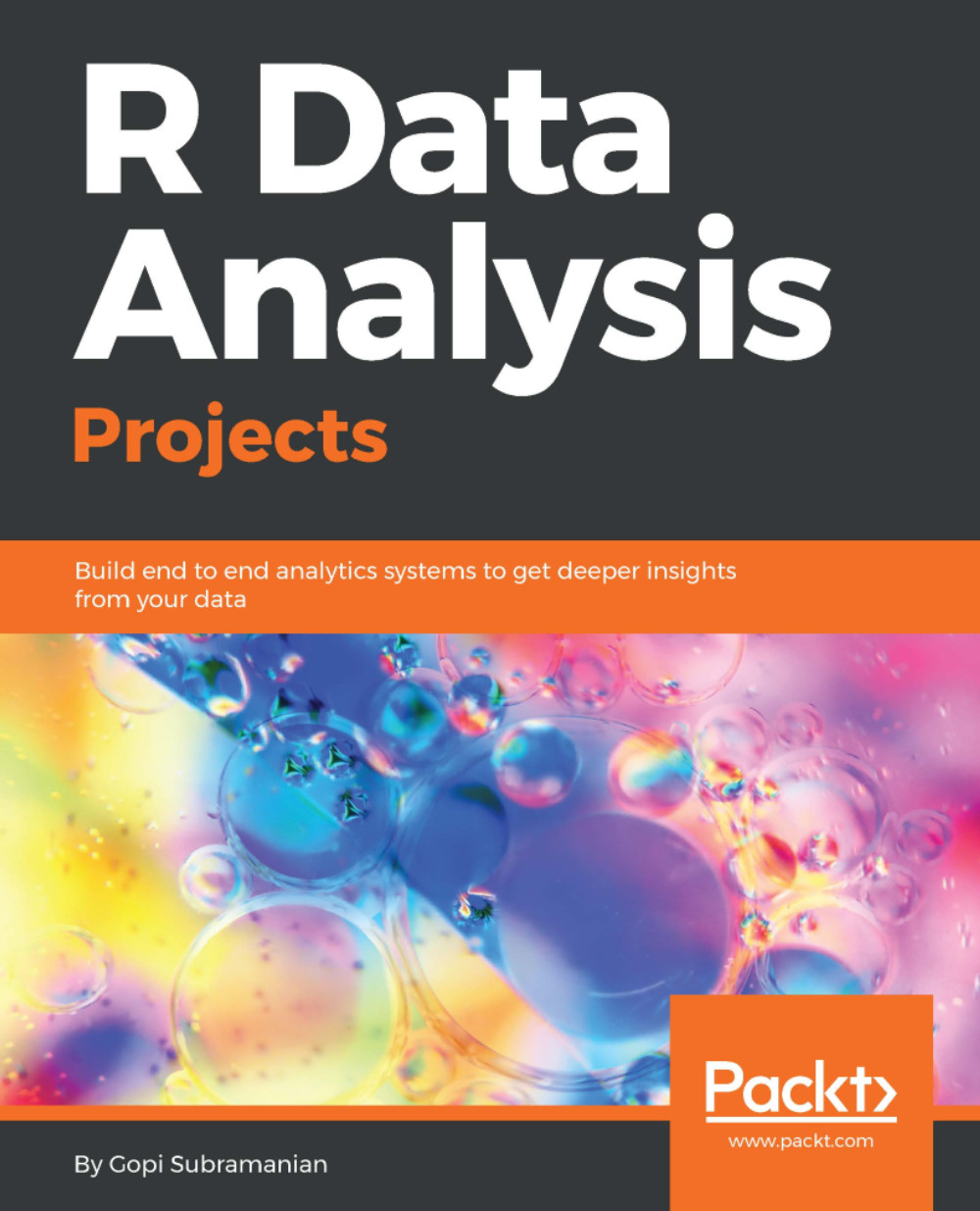
R Data Analysis Projects
€41.99
Data Analysis with R, Second Edition
€32.99
Regression Analysis with R
€32.99
Total 107.97 Stars icon
Banner background image

Table of Contents

18 Chapters
RefresheR Chevron down icon Chevron up icon
The Shape of Data Chevron down icon Chevron up icon
Describing Relationships Chevron down icon Chevron up icon
Probability Chevron down icon Chevron up icon
Using Data To Reason About The World Chevron down icon Chevron up icon
Testing Hypotheses Chevron down icon Chevron up icon
Bayesian Methods Chevron down icon Chevron up icon
The Bootstrap Chevron down icon Chevron up icon
Predicting Continuous Variables Chevron down icon Chevron up icon
Predicting Categorical Variables Chevron down icon Chevron up icon
Predicting Changes with Time Chevron down icon Chevron up icon
Sources of Data Chevron down icon Chevron up icon
Dealing with Missing Data Chevron down icon Chevron up icon
Dealing with Messy Data Chevron down icon Chevron up icon
Dealing with Large Data Chevron down icon Chevron up icon
Working with Popular R Packages Chevron down icon Chevron up icon
Reproducibility and Best Practices Chevron down icon Chevron up icon
Other Books You May Enjoy Chevron down icon Chevron up icon

Customer reviews

Rating distribution
Full star icon Full star icon Full star icon Half star icon Empty star icon 3.5
(2 Ratings)
5 star 50%
4 star 0%
3 star 0%
2 star 50%
1 star 0%
hunterthehunted Aug 07, 2020
Full star icon Full star icon Full star icon Full star icon Full star icon 5
Well written for people at any level of R. Highly recommended for anyone wanting to learn data analytics using R.
Amazon Verified review Amazon
Peter Baker Jul 16, 2021
Full star icon Full star icon Empty star icon Empty star icon Empty star icon 2
I have a good understanding of the R language and wanted a book to bring me forward in the field of Data Analysis... Boy, did I make a mistake."No prior exposure to data analysis is needed, although a fundamental understanding of the R programming language is required to get the best out of this book"This has to be a joke. I have never read a book that leaves you so dam confused even after of 2 chapters I was total unable to figure out what or which way the Author was going. Even the simple things like univariate data description is so long winded as to leave your head reeling.Don't get dragged in NOT for beginners
Amazon Verified review Amazon
Get free access to Packt library with over 7500+ books and video courses for 7 days!
Start Free Trial

FAQs

How do I buy and download an eBook? Chevron down icon Chevron up icon

Where there is an eBook version of a title available, you can buy it from the book details for that title. Add either the standalone eBook or the eBook and print book bundle to your shopping cart. Your eBook will show in your cart as a product on its own. After completing checkout and payment in the normal way, you will receive your receipt on the screen containing a link to a personalised PDF download file. This link will remain active for 30 days. You can download backup copies of the file by logging in to your account at any time.

If you already have Adobe reader installed, then clicking on the link will download and open the PDF file directly. If you don't, then save the PDF file on your machine and download the Reader to view it.

Please Note: Packt eBooks are non-returnable and non-refundable.

Packt eBook and Licensing When you buy an eBook from Packt Publishing, completing your purchase means you accept the terms of our licence agreement. Please read the full text of the agreement. In it we have tried to balance the need for the ebook to be usable for you the reader with our needs to protect the rights of us as Publishers and of our authors. In summary, the agreement says:

  • You may make copies of your eBook for your own use onto any machine
  • You may not pass copies of the eBook on to anyone else
How can I make a purchase on your website? Chevron down icon Chevron up icon

If you want to purchase a video course, eBook or Bundle (Print+eBook) please follow below steps:

  1. Register on our website using your email address and the password.
  2. Search for the title by name or ISBN using the search option.
  3. Select the title you want to purchase.
  4. Choose the format you wish to purchase the title in; if you order the Print Book, you get a free eBook copy of the same title. 
  5. Proceed with the checkout process (payment to be made using Credit Card, Debit Cart, or PayPal)
Where can I access support around an eBook? Chevron down icon Chevron up icon
  • If you experience a problem with using or installing Adobe Reader, the contact Adobe directly.
  • To view the errata for the book, see www.packtpub.com/support and view the pages for the title you have.
  • To view your account details or to download a new copy of the book go to www.packtpub.com/account
  • To contact us directly if a problem is not resolved, use www.packtpub.com/contact-us
What eBook formats do Packt support? Chevron down icon Chevron up icon

Our eBooks are currently available in a variety of formats such as PDF and ePubs. In the future, this may well change with trends and development in technology, but please note that our PDFs are not Adobe eBook Reader format, which has greater restrictions on security.

You will need to use Adobe Reader v9 or later in order to read Packt's PDF eBooks.

What are the benefits of eBooks? Chevron down icon Chevron up icon
  • You can get the information you need immediately
  • You can easily take them with you on a laptop
  • You can download them an unlimited number of times
  • You can print them out
  • They are copy-paste enabled
  • They are searchable
  • There is no password protection
  • They are lower price than print
  • They save resources and space
What is an eBook? Chevron down icon Chevron up icon

Packt eBooks are a complete electronic version of the print edition, available in PDF and ePub formats. Every piece of content down to the page numbering is the same. Because we save the costs of printing and shipping the book to you, we are able to offer eBooks at a lower cost than print editions.

When you have purchased an eBook, simply login to your account and click on the link in Your Download Area. We recommend you saving the file to your hard drive before opening it.

For optimal viewing of our eBooks, we recommend you download and install the free Adobe Reader version 9.