Search icon CANCEL
Subscription
0
Cart icon
Your Cart (0 item)
Close icon
You have no products in your basket yet
Arrow left icon
Explore Products
Best Sellers
New Releases
Books
Videos
Audiobooks
Learning Hub
Conferences
Free Learning
Arrow right icon
Arrow up icon
GO TO TOP
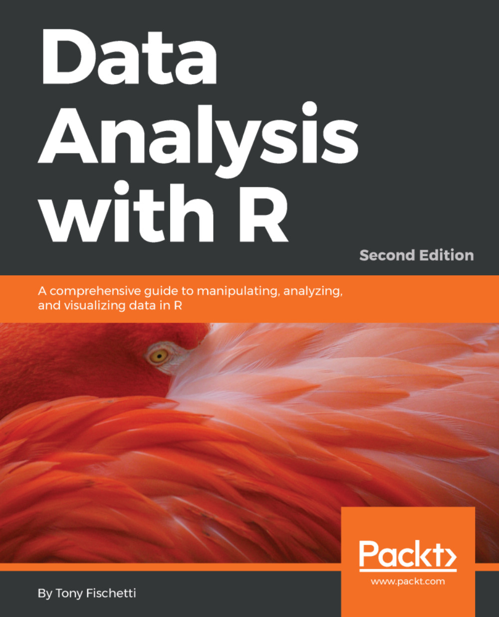
Data Analysis with R, Second Edition

You're reading from   Data Analysis with R, Second Edition A comprehensive guide to manipulating, analyzing, and visualizing data in R

Arrow left icon
Product type Paperback
Published in Mar 2018
Publisher Packt
ISBN-13 9781788393720
Length 570 pages
Edition 2nd Edition
Languages
Tools
Arrow right icon
Author (1):
Arrow left icon
Tony Fischetti Tony Fischetti
Author Profile Icon Tony Fischetti
Tony Fischetti
Arrow right icon
View More author details
Toc

Table of Contents (19) Chapters Close

Preface 1. RefresheR FREE CHAPTER 2. The Shape of Data 3. Describing Relationships 4. Probability 5. Using Data To Reason About The World 6. Testing Hypotheses 7. Bayesian Methods 8. The Bootstrap 9. Predicting Continuous Variables 10. Predicting Categorical Variables 11. Predicting Changes with Time 12. Sources of Data 13. Dealing with Missing Data 14. Dealing with Messy Data 15. Dealing with Large Data 16. Working with Popular R Packages 17. Reproducibility and Best Practices 18. Other Books You May Enjoy

Vectors

Vectors are the most basic data structures in R, and they are ubiquitous indeed. In fact, even the single values that we've been working with thus far were actually vectors of length 1. That's why the interactive R console has been printing [1] along with all of our output.

Vectors are essentially an ordered collection of values of the same atomic data type. Vectors can be arbitrarily large (with some limitations) or they can be just one single value.

The canonical way of building vectors manually is using the c() function (which stands for combine):

  > our.vect <- c(8, 6, 7, 5, 3, 0, 9) 
  > our.vect 
  [1] 8 6 7 5 3 0 9 

In the preceding example, we created a numeric vector of length 7 (namely, Jenny's telephone number).

Let's try to put character data types into this vector as follows:

  > another.vect <- c("8", 6, 7, "-", 3, "0", 9) 
  > another.vect 
  [1] "8" "6" "7" "-" "3" "0" "9" 

R would convert all the items in the vector (called elements) into character data types to satisfy the condition that all elements of a vector must be of the same type. A similar thing happens when you try to use logical values in a vector with numbers; the logical values would be converted into 1 and 0 (for TRUE and FALSE, respectively). These logicals will turn into TRUE and FALSE (note the quotation marks) when used in a vector that contains characters.

Subsetting

It is very common to want to extract one or more elements from a vector. For this, we use a technique called indexing or subsetting. After the vector, we put an integer in square brackets ([]) called the subscript operator. This instructs R to return the element at that index. The indices (plural for index, in case you were wondering!) for vectors in R start at 1 and stop at the length of the vector:

  > our.vect[1]                  # to get the first value 
  [1] 8 
  > # the function length() returns the length of a vector 
  > length(our.vect) 
  [1] 7 
  > our.vect[length(our.vect)]   # get the last element of a vector 
  [1] 9 

Note that in the preceding code, we used a function in the subscript operator. In cases like these, R evaluates the expression in the subscript operator and uses the number it returns as the index to extract.

If we get greedy and try to extract an element from an index that doesn't exist, R will respond with NA, meaning, not available. We see this special value cropping up from time to time throughout this text:

  > our.vect[10] 
  [1] NA 

One of the most powerful ideas in R is that you can use vectors to subset other vectors:

  > # extract the first, third, fifth, and 
  > # seventh element from our vector 
  > our.vect[c(1, 3, 5, 7)] 
  [1] 8 7 3 9 

The ability to use vectors to index other vectors may not seem like much now, but its usefulness will become clear soon.

Another way to create vectors is using sequences:

  > other.vector <- 1:10 
  > other.vector 
  [1]  1  2  3  4  5  6  7  8  9 10 
  > another.vector <- seq(50, 30, by=-2) 
  > another.vector 
  [1] 50 48 46 44 42 40 38 36 34 32 30 

Here, the 1:10 statement creates a vector from 1 to 10. 10:1 would have created the same 10-element vector, but in reverse. The seq() function is more general in that it allows sequences to be made using steps (among many other things).

Combining our knowledge of sequences and vectors subsetting vectors, we can get the first five digits of Jenny's number:

  > our.vect[1:5] 
  [1] 8 6 7 5 3 

Vectorized functions

Part of what makes R so powerful is that many of R's functions take vectors as arguments. These vectorized functions are usually extremely fast and efficient. We've already seen one such function, length(), but there are many, many others:

  > # takes the mean of a vector 
  > mean(our.vect) 
  [1] 5.428571 
  > sd(our.vect)    # standard deviation 
  [1] 3.101459 
  > min(our.vect) 
  [1] 0 
  > max(1:10) 
  [1] 10 
  > sum(c(1, 2, 3)) 
  [1] 6 

In practical settings, such as when reading data from files, it is common to have NA values in vectors:

  > messy.vector <- c(8, 6, NA, 7, 5, NA, 3, 0, 9) 
  > messy.vector 
  [1]  8  6 NA  7  5 NA  3  0  9 
  > length(messy.vector) 
  [1] 9 

Some vectorized functions will not allow NA values by default. In these cases, an extra keyword argument must be supplied along with the first argument to the function:

  > mean(messy.vector) 
  [1] NA 
  > mean(messy.vector, na.rm=TRUE) 
  [1] 5.428571 
  > sum(messy.vector, na.rm=FALSE) 
  [1] NA 
  > sum(messy.vector, na.rm=TRUE) 
  [1] 38 

As mentioned previously, vectors can be constructed from logical values as well:

  > log.vector <- c(TRUE, TRUE, FALSE) 
  > log.vector 
  [1]  TRUE TRUE FALSE 

Since logical values can be coerced into behaving like numerics, as we saw earlier, if we try to sum a logical vector as follows:

  > sum(log.vector) 
  [1] 2 

We will, essentially, get a count of the number of TRUE values in that vector.

There are many functions in R that operate on vectors and return logical vectors. is.na() is one such function. It returns a logical vector, that is, the same length as the vector supplied as an argument, with a TRUE in the position of every NA value. Remember our messy vector (from just a minute ago)?

  > messy.vector 
  [1]  8  6 NA  7  5 NA  3  0  9 
  > is.na(messy.vector) 
  [1] FALSE FALSE  TRUE FALSE FALSE  TRUE FALSE FALSE FALSE 
  > #  8     6      NA   7     5      NA   3       0    9 

Putting together these pieces of information, we can get a count of the number of NA values in a vector as follows:

  > sum(is.na(messy.vector)) 
  [1] 2 

When you use Boolean operators on vectors, they also return logical vectors of the same length as the vector being operated on:

  > our.vect > 5 
  [1]  TRUE  TRUE  TRUE FALSE FALSE FALSE  TRUE 

If we wanted to--and we do--count the number of digits in Jenny's phone number that are greater than five, we would do so in the following manner:

  > sum(our.vect > 5) 
  [1] 4 

Advanced subsetting

Did I mention that we can use vectors to subset other vectors! When we subset vectors using logical vectors of the same length, only the elements corresponding to the TRUE values are extracted. Hopefully, light bulbs are starting to go off in your head. If we wanted to extract only the legitimate non-NA digits from Jenny's number, we can do it as follows:

  > messy.vector[!is.na(messy.vector)] 
  [1] 8 6 7 5 3 0 9 

This is a very critical trait of R, so let's take our time understanding it; this idiom will come up again and again throughout this book.

The logical vector that yields TRUE when an NA value occurs in messy.vector (from is.na()) is then negated (the whole thing) by the negation operator,  !. The resultant vector is TRUE whenever the corresponding value in messy.vector is not NA. When this logical vector is used to subset the original messy vector, it only extracts the non-NA values from it.

Similarly, we can show all the digits in Jenny's phone number that are greater than five as follows:

  > our.vect[our.vect > 5] 
  [1] 8 6 7 9 

Thus far, we've only been displaying elements that have been extracted from a vector. However, just as we've been assigning and reassigning variables, we can assign values to various indices of a vector and change the vector as a result. For example, if Jenny tells us that we have the first digit of her phone number wrong (it's really 9), we can reassign just that element without modifying the others:

  > our.vect 
  [1] 8 6 7 5 3 0 9 
  > our.vect[1] <- 9 
  > our.vect 
  [1] 9 6 7 5 3 0 9 

Sometimes, it may be required to replace all the NA values in a vector with the value 0. To do this with our messy vector, we can execute the following command:

  > messy.vector[is.na(messy.vector)] <- 0 
  > messy.vector 
  [1] 8 6 0 7 5 0 3 0 9 

Elegant though the preceding solution is, modifying a vector in place is usually discouraged in favor of creating a copy of the original vector and modifying the copy. One such technique to perform this is using the ifelse() function.

Not to be confused with the if/else control construct, ifelse() is a function that takes three arguments: a test that returns a logical/Boolean value, a value to use if the element passes the test, and one to return if the element fails the test.

The preceding in-place modification solution could be reimplemented with ifelse as follows:

  > ifelse(is.na(messy.vector), 0, messy.vector) 
  [1] 8 6 0 7 5 0 3 0 9 

Recycling

The last important property of vectors and vector operations in R is that they can be recycled. To understand what I mean, examine the following expression:

  > our.vect + 3 
  [1] 12  9 10  8  6  3 12 

This expression adds three to each digit in Jenny's phone number. Although it may look so, R is not performing this operation between a vector and a single value. Remember when I said that single values are actually vectors of the length 1? What is really happening here is that R is told to perform element-wise addition on a vector of length 7 and a vector of length 1. As element-wise addition is not defined for vectors of differing lengths, R recycles the smaller vector until it reaches the same length as that of the bigger vector. Once both the vectors are the same size, then R, element by element, performs the addition and returns the result:

  > our.vect + 3 
  [1] 12  9 10  8  6  3 12 

This is tantamount to the following:

  > our.vect + c(3, 3, 3, 3, 3, 3, 3) 
  [1] 12  9 10  8  6  3 12 

If we wanted to extract every other digit from Jenny's phone number, we can do so in the following manner:

  > our.vect[c(TRUE, FALSE)] 
  [1] 9 7 3 9 

This works because the vector c(TRUE, FALSE) is repeated until it is of the length 7, making it equivalent to the following:

  > our.vect[c(TRUE, FALSE, TRUE, FALSE, TRUE, FALSE, TRUE)] 
  [1] 9 7 3 9 

One common snag related to vector recycling that R users (useRs, if I may) encounter is that during some arithmetic operations involving vectors of discrepant length, R will warn you if the smaller vector cannot be repeated a whole number of times to reach the length of the bigger vector. This is not a problem when doing vector arithmetic with single values as 1 can be repeated any number of times to match the length of any vector (which must, of course, be an integer). It would pose a problem, though, if we were looking to add three to every other element in Jenny's phone number:

  > our.vect + c(3, 0) 
  [1] 12  6 10  5  6  0 12 
  Warning message: 
  In our.vect + c(3, 0) : 
    longer object length is not a multiple of shorter object length 

You will likely learn to love these warnings as they have stopped many useRs from making grave errors.

Before we move on to the next section, an important thing to note is that in a lot of other programming languages, many of the things that we did would have been implemented using for loops and other control structures. Although there is certainly a place for loops and such in R, often a more sophisticated solution exists in using just vector/matrix operations. In addition to elegance and brevity, the solution that exploits vectorization and recycling is often much more efficient.

You have been reading a chapter from
Data Analysis with R, Second Edition - Second Edition
Published in: Mar 2018
Publisher: Packt
ISBN-13: 9781788393720
Register for a free Packt account to unlock a world of extra content!
A free Packt account unlocks extra newsletters, articles, discounted offers, and much more. Start advancing your knowledge today.
Unlock this book and the full library FREE for 7 days
Get unlimited access to 7000+ expert-authored eBooks and videos courses covering every tech area you can think of
Renews at $19.99/month. Cancel anytime
Banner background image