Exploring basic networking

Today, it’s almost inconceivable to imagine a computer not connected to some sort of network or the internet. Our ever-increasing online presence, cloud computing, mobile communications, and Internet of Things (IoT) would not be possible without the highly distributed, high-speed, and scalable networks serving the underlying data traffic; yet the basic networking principles behind the driving force of the modern-day internet are decades old. Networking and communication paradigms will continue to evolve, but some of the original primitives and concepts will still have a long-lasting effect in shaping the building blocks of future communications.

This section will introduce you to a few of these networking essentials and, hopefully, spark your curiosity for further exploration. Let’s start with computer networks.

Computer networks

A computer network is a group of two or more computers (or nodes) connected via a physical medium (cable, wireless, optical) and communicating with each other using a standard set of agreed-upon communication protocols. At a very high level, a network communication infrastructure includes computers, devices, switches, routers, Ethernet or optical cables, wireless environments, and all sorts of network equipment.

Beyond the physical connectivity and arrangement, networks are also defined by a logical layout via network topologies, tiers, and the related data flow. An example of a logical networking hierarchy is the three-tiered layering of the demilitarized zone (DMZ), firewall, and internal networks. The DMZ is an organization’s outward-facing network, with an extra security layer against the public internet. A firewall controls the network traffic between the DMZ and the internal network.

Network devices are identified by the following aspects:

• Network addresses: These assist with locating nodes on the network using communication protocols, such as the Internet Protocol (IP) (see more on IP in the TCP/IP protocols section, later in this chapter)
• Hostnames: These are user-friendly labels associated with devices that are easier to remember than network addresses

A common classification criterion looks at the scale and expansion of computer networks. Let’s introduce you to local area networks (LANs) and wide area networks (WANs):

• LANs: A LAN represents a group of devices connected and located in a single physical location, such as a private residence, school, or office. A LAN can be of any size, ranging from a home network with only a few devices to large-scale enterprise networks with thousands of users and computers.

  Regardless of the network’s size, a LAN’s essential characteristic is that it connects devices in a single, limited area. Examples of LANs include the home network of a single-family residence or your local coffee shop’s free wireless service.

  For more information about LANs, you can refer to https://www.cisco.com/c/en/us/products/switches/what-is-a-lan-local-area-network.html.

  When a computer network spans multiple regions or multiple interconnected LANs, WANs come into play.

• WANs: A WAN is usually a network of networks, with multiple or distributed LANs communicating with each other. In this sense, we regard the internet as the world’s largest WAN. An example of a WAN is the computer network of a multinational company’s geographically distributed offices worldwide. Some WANs are built by service providers, to be leased to various businesses and institutions around the world.

  WANs have several variations, depending on their type, range, and use. Typical examples of WANs include personal area networks (PANs), metropolitan area networks (MANs), and cloud or internet area networks (IANs).

  For more information about WANs, you can refer to https://www.cisco.com/c/en/us/products/switches/what-is-a-wan-wide-area-network.html.

We think that an adequate introduction to basic networking principles should always include a brief presentation of the theoretical model governing network communications in general. We’ll look at this next.

The OSI model

The Open Systems Interconnection (OSI) model is a theoretical representation of a multilayer communication mechanism between computer systems interacting over a network. The OSI model was introduced in 1983 by the International Organization for Standardization (ISO) to provide a standard for different computer systems to communicate with each other.

We can regard the OSI model as a universal framework for network communications. As the following figure shows, the OSI model defines a stack of seven layers, directing the communication flow:

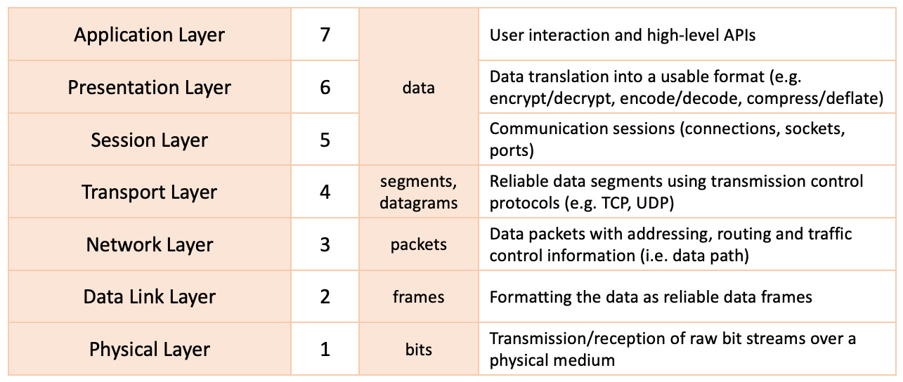
Figure 7.1 – The OSI model

In the layered view shown in the preceding figure, the communication flow moves from top to bottom (on the transmitting end) or bottom to top (on the receiving end). Before we look at each layer in more detail, let’s briefly explain how the OSI model and data encapsulation and decapsulation work.

Data encapsulation and decapsulation in the OSI model

When using the network to transfer data from one computer to another, some specific rules are followed. Inside the OSI model, the network data flows in two different ways. One way is down, from Layer 7 to Layer 1, and this is known as data encapsulation. The other way, up from Layer 1 to Layer 7, is known as data decapsulation. Data encapsulation represents the process of sending data from one computer to another, while data decapsulation represents the process of receiving data. Let’s look at these in greater detail:

• Encapsulation: When sending data, data from one computer is converted to be sent through the network, and it receives extra information as it is being sent though all the layers of the stack. The application layer (Layer 7) is the place where the user directly interacts with the application. Then, data is sent through the presentation (Layer 6) and session (Layer 5) layers, where data is transformed into a usable format. In the transport layer (Layer 4), data is broken into smaller chunks (segments) and receives a new TCP header. Inside the network layer (Layer 3), the data is called a packet, receives an IP header, and is sent to the data link layer (Layer 2), where it is called a frame and contains both TCP and IP headers. At Layer 2, each frame receives information about the hardware addresses of the source and destination (media access control (MAC) addresses) and information about the protocols to be used in the network layer (created by the logical link control (LLC) data communication protocol). At this point, a new field is added, called Frame Check Sequence (FCS), which is used for checking errors. Then, the frames are passed through the physical layer (Layer 1).
• Decapsulation: When data is received, the process is identical, but in reverse order. This starts from the physical layer (Layer 1), where the first synchronization happens, after which the frame is sent through the data link layer (Layer 2), where an error check is done, by verifying the FCS field. This process is called a Cyclic Redundancy Check (CRC). The data, which is now a packet, is sent through all the other layers. Here, the headers that were added during the encapsulation process are stripped off until they reach the upper layers and become ready to be used on the target computer. A graphic explanation is provided in the following figure:

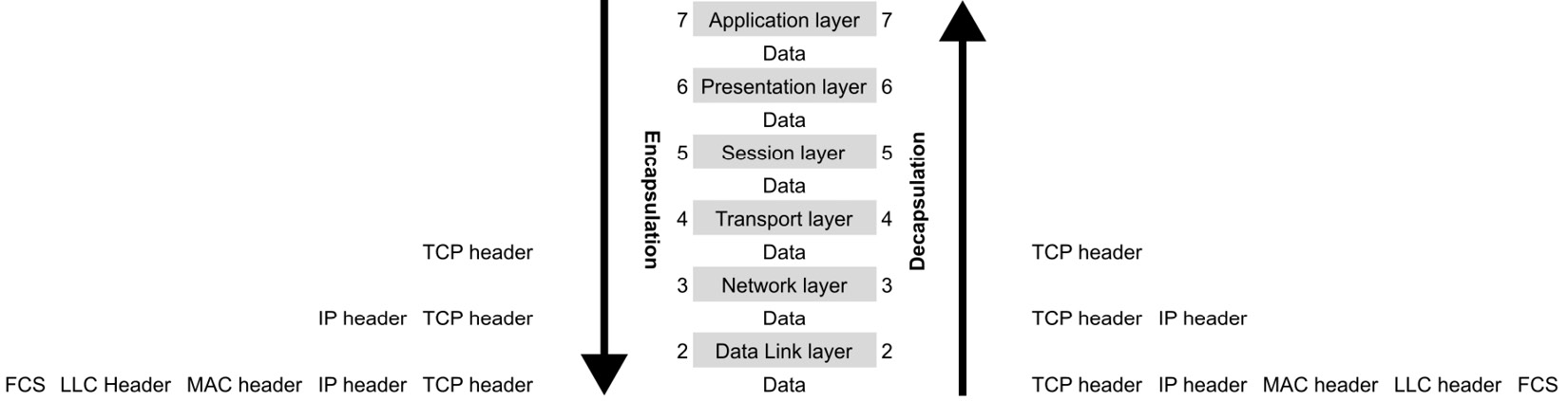
Figure 7.2 – Encapsulation and decapsulation in the OSI model

Let’s look at each of these layers in detail and describe their functionality in shaping network communication.

The physical layer

The physical layer (or Layer 1) consists of the networking equipment or infrastructure connecting the devices and serving the communication, such as cables, wireless or optical environments, connectors, and switches. This layer handles the conversion between raw bit streams and the communication medium (which includes electrical, radio, or optical signals) while regulating the corresponding bit-rate control.

Examples of protocols operating at the physical layer include Ethernet, Universal Serial Bus (USB), and Digital Subscriber Line (DSL).

The data link layer

The data link layer (or Layer 2) establishes a reliable data flow between two directly connected devices on a network, either as adjacent nodes in a WAN or as devices within a LAN. One of the data link layer’s responsibilities is flow control, adapting to the physical layer’s communication speed. On the receiving device, the data link layer corrects communication errors that originated in the physical layer. The data link layer consists of the following subsystems:

• Media access control (MAC): This subsystem uses MAC addresses to identify and connect devices on the network. It also controls the device access permissions to transmit and receive data on the network.
• Logical link control (LLC): This subsystem identifies and encapsulates network layer protocols and performs error checking and frame synchronization while transmitting or receiving data.

The protocol data units controlled by the data link layer are also known as frames. A frame is a data transmission unit that acts as a container for a single network packet. Network packets are processed at the next OSI level (network layer). When multiple devices access the same physical layer simultaneously, frame collisions may occur. Data link layer protocols can detect and recover from such collisions and further reduce or prevent their occurrence.

There are also Ethernet frames, for example, which are encapsulated data that is defined for MAC implementations. The original IEEE 802.3 Ethernet format, the 802.3 SubNetwork Access Protocol (SNAP), and the Ethernet II (extended) frame formats are also available.

One more example of the data link protocol is the Point-to-Point Protocol (PPP), a binary networking protocol that’s used in high-speed broadband communication networks.

The network layer

The network layer (or Layer 3) discovers the optimal communication path (or route) between devices on a network. This layer uses a routing mechanism based on the IP addresses of the devices involved in the data exchange to move data packets from source to destination.

On the transmitting end, the network layer disassembles the data segments that originated in the transport layer into network packets. On the receiving end, the data frames are reassembled from the layer below (data link layer) into packets.

A protocol that operates at the network layer is the Internet Control Message Protocol (ICMP). ICMP is used by network devices to diagnose network communication issues. ICMP reports an error when a requested endpoint is not available by sending messages such as destination network unreachable, timer expired, source route failed, and others.

The transport layer

The transport layer (or Layer 4) operates with data segments or datagrams. This layer is mainly responsible for transferring data from a source to a destination and guaranteeing a specific quality of service (QoS). On the transmitting end, data that originated from the layer above (session layer) is disassembled into segments. On the receiving end, the transport layer reassembles the data packets received from the layer below (network layer) into segments.

The transport layer maintains the reliability of the data transfer through flow-control and error-control functions. The flow-control function adjusts the data transfer rate between endpoints with different connection speeds, to avoid a sender overwhelming the receiver. When the data received is incorrect, the error-control function may request the retransmission of data.

Examples of transport layer protocols include the Transmission Control Protocol (TCP) and the User Datagram Protocol (UDP).

The session layer

The session layer (or Layer 5) controls the lifetime of the connection channels (or sessions) between devices communicating on a network. At this layer, sessions or network connections are usually defined by network addresses, sockets, and ports. We’ll explain each of these concepts in the Sockets and ports and IP addresses sections. The session layer is responsible for the integrity of the data transfer within a communication channel or session. For example, if a session is interrupted, the data transfer resumes from a previous checkpoint.

Some typical session layer protocols are the Remote Procedure Call (RPC) protocol, which is used by interprocess communications, and Network Basic Input/Output System (NetBIOS), which is a file-sharing and name-resolution protocol.

The presentation layer

The presentation layer (or Layer 6) acts as a data translation tier between the application layer above and the session layer below. On the transmitting end, this layer formats the data into a system-independent representation before sending it across the network. On the receiving end, the presentation layer transforms the data into an application-friendly format. Examples of such transformations are encryption and decryption, compression and decompression, encoding and decoding, and serialization and deserialization.

Usually, there is no substantial distinction between the presentation and application layers, mainly due to the relatively tight coupling of the various data formats with the applications consuming them. Standard data representation formats include the American Standard Code for Information Interchange (ASCII), Extensible Markup Language (XML), JavaScript Object Notation (JSON), Joint Photographic Experts Group (JPEG), ZIP, and others.

The application layer

The application layer (or Layer 7) is the closest to the end user in the OSI model. This layer collects or provides the input or output of application data in some meaningful way. This layer does not contain or run the applications themselves. Instead, it acts as an abstraction between applications, implementing a communication component and the underlying network. Typical examples of applications that interact with the application layer are web browsers and email clients.

A few examples of Layer 7 protocols are the DNS protocol, the HyperText Transfer Protocol (HTTP), the File Transfer Protocol (FTP), and email messaging protocols, such as the Post Office Protocol (POP), Internet Message Access Protocol (IMAP), and Simple Mail Transfer Protocol (SMTP).

Before wrapping up, we should note that the OSI model is a generic representation of networking communication layers and provides the theoretical guidelines for how network communication works. A similar – but more practical – illustration of the networking stack is the TCP/IP model. Both these models are useful when it comes to network design, implementation, troubleshooting, and diagnostics. The OSI model gives network operators a good understanding of the full networking stack, from the physical medium to the application layer, and each level has Protocol Data Units (PDUs) and communication internals. However, the TCP/IP model is somewhat simplified, with a few of the OSI model layers collapsed into one, and it takes a rather protocol-centric approach to network communications. We’ll explore this in more detail in the next section.

The TCP/IP network stack model

The TCP/IP model is a four-layer interpretation of the OSI networking stack, where some of the equivalent OSI layers appear consolidated, as shown in the following figure:

Figure 7.3 – The OSI and TCP/IP models

Chronologically, the TCP/IP model is older than the OSI model. It was first suggested by the US Department of Defense (DoD) as part of an internetwork project developed by the Defense Advanced Research Projects Agency (DARPA). This project eventually became the modern-day internet.

The TCP/IP model layers encapsulate similar functions to their counterpart OSI layers. Here’s a summary of each layer in the TCP/IP model.

The network interface layer

The network interface layer is responsible for data delivery over a physical medium (such as wire, wireless, or optical). Networking protocols operating at this layer include Ethernet, Token Ring, and Frame Relay. This layer maps to the composition of the physical and data link layers in the OSI model.

The internet layer

The internet layer provides connectionless data delivery between nodes on a network. Connectionless protocols describe a network communication pattern where a sender transmits data to a receiver without a prior arrangement between the two. This layer is responsible for disassembling data into network packets at the transmitting end and reassembling them on the receiving end. The internet layer uses routing functions to identify the optimal path between the network nodes. This layer maps to the network layer in the OSI model.

The transport layer

The transport layer (also known as the transmission layer or the host-to-host layer) is responsible for maintaining the communication sessions between connected network nodes. The transport layer implements error-detection and correction mechanisms for reliable data delivery between endpoints. This layer maps to the transport layer in the OSI model.

The application layer

The application layer provides the data communication abstraction between software applications and the underlying network. This layer maps to the composition of the session, presentation, and application layers in the OSI model.

As discussed earlier in this chapter, the TCP/IP model is a protocol-centric representation of the networking stack. This model served as the foundation of the internet by gradually defining and developing networking protocols required for internet communications. These protocols are collectively referred to as the IP suite. The following section describes some of the most common networking protocols.

TCP/IP protocols

In this section, we’ll describe some widely used networking protocols. The reference provided here should not be regarded as an all-encompassing guide. There are a vast number of TCP/IP protocols, and a comprehensive study is beyond the scope of this chapter. Nevertheless, there are a handful of protocols worth exploring, frequently at work in everyday network communication and administration workflows.

The following list briefly describes each TCP/IP protocol and its related Request for Comments (RFC) identifier. The RFC represents the detailed technical documentation – of a protocol, in our case – that’s usually authored by the Internet Engineering Task Force (IETF). For more information about RFC, please refer to https://www.ietf.org/standards/rfcs/. Here are the most widely used protocols:

• IP: IP (RFC 791) identifies network nodes based on fixed-length addresses, also known as IP addresses. IP addresses will be described in more detail in the next section. The IP protocol uses datagrams as the data transmission unit and provides fragmentation and reassembly capabilities of large datagrams to accommodate small-packet networks (and avoid transmission delays). The IP protocol also provides routing functions to find the optimal data path between network nodes. IP operates at the network layer (Layer 3) in the OSI model.
• ARP: The Address Resolution Protocol (ARP) (RFC 826) is used by the IP protocol to map IP network addresses (specifically, IP version 4 or IPv4) to device MAC addresses used by a data link protocol. ARP operates at the data link layer (Layer 2) in the OSI model.
• NDP: The Neighbor Discovery Protocol (NDP) (RFC 4861) is like the ARP protocol, and it also controls IP version 6 (IPv6) address mapping. NDP operates within the data link layer (Layer 2) in the OSI model.
• ICMP: ICMP (RFC 792) is a supporting protocol for checking transmission issues. When a device or node is not reachable within a given timeout, ICMP reports an error. ICMP operates at the network layer (Layer 3) in the OSI model.
• TCP: TCP (RFC 793) is a connection-oriented, highly reliable communication protocol. TCP requires a logical connection (such as a handshake) between the nodes before initiating the data exchange. TCP operates at the transport layer (Layer 4) in the OSI model.
• UDP: UDP (RFC 768) is a connectionless communication protocol. UDP has no handshake mechanism (compared to TCP). Consequently, with UDP, there’s no guarantee of data delivery. It is also known as a best-effort protocol. UDP uses datagrams as the data transmission unit, and it’s suitable for network communications where error checking is not critical. UDP operates at the transport layer (Layer 4) in the OSI model.
• Dynamic Host Configuration Protocol (DHCP): The DHCP (RFC 2131) provides a framework for requesting and passing host configuration information required by devices on a TCP/IP network. DHCP enables the automatic (dynamic) allocation of reusable IP addresses and other configuration options. DHCP is considered an application layer (Layer 7) protocol in the OSI model, but the initial DHCP discovery mechanism operates at the data link layer (Layer 2).
• Domain Name System (DNS): The DNS (RFC 2929) is a protocol that acts as a network address book, where nodes in the network are identified by human-readable names instead of IP addresses. According to the IP protocol, each device on a network is identified by a unique IP address. When a network connection specifies the remote device’s hostname (or domain name) before the connection is established, DNS translates the domain name (such as dns.google.com) into an IP address (such as 8.8.8.8). The DNS protocol operates at the application layer (Layer 7) in the OSI model.
• HTTP: HTTP (RFC 2616) is the vehicular language of the internet. HTTP is a stateless application-level protocol based on the request and response between a client application (for example, a browser) and a server endpoint (for example, a web server). HTTP supports a wide variety of data formats, ranging from text to images and video streams. HTTP operates at the application layer (Layer 7) in the OSI model.
• FTP: FTP (RFC 959) is a standard protocol for transferring files requested by an FTP client from an FTP server. FTP operates at the application layer (Layer 7) in the OSI model.
• TELNET: The Terminal Network protocol (TELNET) (RFC 854) is an application-layer protocol that provides a bidirectional text-oriented network communication between a client and a server machine, using a virtual terminal connection. TELNET operates at the application layer (Layer 7) in the OSI model.
• SSH: Secure Shell (SSH) (RFC 4253) is a secure application-layer protocol that encapsulates strong encryption and cryptographic host authentication. SSH uses a virtual terminal connection between a client and a server machine. SSH operates at the application layer (Layer 7) in the OSI model.
• SMTP: SMTP (RFC 5321) is an application-layer protocol for sending and receiving emails between an email client (for example, Outlook) and an email server (such as Exchange Server). SMTP supports strong encryption and host authentication. SMTP acts at the application layer (Layer 7) in the OSI model.
• SNMP: The Simple Network Management Protocol (SNMP) (RFC 1157) is used for remote device management and monitoring. SNMP operates at the application layer (Layer 7) in the OSI model.
• NTP: The Network Time Protocol (NTP) (RFC 5905) is an internet protocol that’s used for synchronizing the system clock of multiple machines across a network. NTP operates at the application layer (Layer 7) in the OSI model.

Most of the internet protocols enumerated previously use the IP protocol to identify devices participating in the communication. Devices on a network are uniquely identified by an IP address. Let’s examine these network addresses more closely.

IP addresses

An IP address is a fixed-length unique identifier (UID) of a device in a network. Devices locate and communicate with each other based on IP addresses. The concept of an IP address is very similar to a postal address of a residence, whereby mail or a package would be sent to that destination based on its address.

Initially, IP defined the IP address as a 32-bit number known as an IPv4 address. With the growth of the internet, the total number of IP addresses in a network has been exhausted. To address this issue, a new version of the IP protocol devised a 128-bit numbering scheme for IP addresses. A 128-bit IP address is also known as an IPv6 address.

In the next few sections, we’ll take a closer look at the networking constructs that play an important role in IP addresses, such as IPv4 and IPv6 address formats, network classes, subnetworks, and broadcast addresses.

IPv4 addresses

An IPv4 address is a 32-bit number (4 bytes) usually expressed as four groups of 1-byte (8 bits) numbers, separated by a dot (.). Each number in these four groups is an integer between 0 and 255. An example of an IPv4 address is 192.168.1.53.

The following figure shows a binary representation of an IPv4 address:

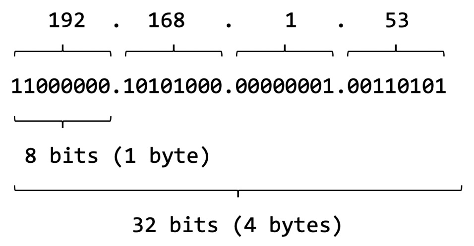
Figure 7.4 – Network classes

The IPv4 address space is limited to 4,294,967,296 (2^32) addresses (roughly 4 billion). Of these, approximately 18 million are reserved for special purposes (for example, private networks), and about 270 million are multicast addresses.

A multicast address is a logical identifier of a group of IP addresses. For more information on multicast addresses, please refer to RFC 6308 (https://tools.ietf.org/html/rfc6308).

Network classes

In the early stages of the internet, the highest-order byte (first group) in the IPv4 address indicated the network number. The subsequent bytes further express the network hierarchy and subnetworks, with the lowest-order byte identifying the device itself. This scheme soon proved insufficient for network hierarchies and segregations as it only allowed for 256 (2^8) networks, denoted by the leading byte of the IPv4 address. As additional networks were added, each with its own identity, the IP address specification needed a special revision to accommodate a standard model. The Classful Network specification, which was introduced in 1981, addressed this problem by dividing the IPv4 address space into five classes based on the leading 4 bits of the address, as illustrated in the following figure:

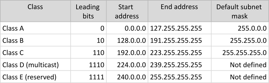
Figure 7.5 – Network classes

For more information on network classes, please refer to RFC 870 (https://tools.ietf.org/html/rfc870). In the preceding figure, the last column specifies the default subnet mask for each of these network classes. We’ll look at subnets (or subnetworks) next.

Subnetworks

Subnetworks (or subnets) are logical subdivisions of an IP network. Subnets were introduced to identify devices that belong to the same network. The IP addresses of devices in the same network have an identical most-significant group. The subnet definition yields a logical division of an IP address into two fields: the network identifier and the host identifier. The numerical representation of the subnet is called a subnet mask or netmask. The following figure provides an example of a network identifier and a host identifier:

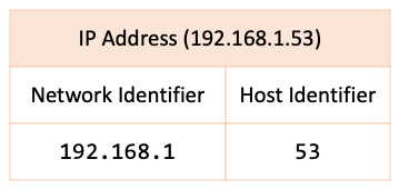
Figure 7.6 – Subnet with network and host identifiers

With our IPv4 address (192.168.1.53), we could devise a network identifier of 192.168.1, where the host identifier is 53. The resulting subnet mask would be as follows:

192.168.1.0

We dropped the least significant group in the subnet mask, representing the host identifier (53), and replaced it with 0. Here, 0 indicates the starting address in the subnet. In other words, any host identifier value in the range of 0 to 255 is allowed in the subnetwork. For example, 192.168.1.92 is a valid (and accepted) IP address in the 192.168.1.0 network.

An alternative representation of subnets uses so-called Classless Inter-Domain Routing (CIDR) notation. CIDR represents an IP address as the network address (prefix) followed by a slash (/) and the bit-length of the prefix. In our case, the CIDR notation of the 192.168.1.0 subnet is this:

192.168.1.0/24

The first three groups in the network address make up 3 x 8 = 24 bits, hence the /24 notation.

Usually, subnets are planned with the host identifier address as a starting point. Back to our example, suppose we wanted our host identifier addresses in the network to start with 100 and end with 125. Let’s look at how we can achieve this.

First, let’s see the binary representation of 192.168.1.100:

11000000.10101000.00000001.01100100

As you can see, the last group, highlighted in the preceding sequence, represents the host identifier (100). Remember that we want the network to start with 100 and end with 125. This means that the closest binary value to the reserved 99 addresses that would not be permitted in our subnet is 96 = 64 + 32. The equivalent binary value for it is as follows:

11100000

In other words, the three most significant bits in the host identifier are reserved. Reserved bits in the subnet representation are shown as 1. These bits would be added to the 24 already reserved bits of the network address (192.168.1), accounting in total for 27 = 24 + 3 bits. Here’s the equivalent representation:

11111111.11111111.11111111.11100000

Consequently, the resulting netmask is as follows:

255.255.255.224

The CIDR notation of the corresponding subnet is shown here:

192.168.1.96/27

The remaining five bits in the host identifier’s group account for 2^5 = 32 possible addresses in the subnet, starting with 97. This would limit the maximum host identifier value to 127 = 96 + 32 – 1 (we subtract 1 to account for the starting number of 97 included in the total of 32). In this range of 32 addresses, the last IP address is reserved as a broadcast address, as shown here:

192.168.1.127

A broadcast address is reserved as the highest number in a network or subnet, when applicable. Back to our example, excluding the broadcast address, the maximum host IP address in the subnet is as follows:

192.168.1.126

You can learn more about subnets in RFC 1918 (https://tools.ietf.org/html/rfc1918). Since we mentioned the broadcast address, let’s have a quick look at it.

Broadcast addresses

A broadcast address is a reserved IP address in a network or subnetwork that’s used to transmit a collective message (data) to all devices belonging to the network. The broadcast address is the last IP address in the network or subnet, when applicable.

For example, the broadcast address of the 192.168.1.0/24 network is 192.168.1.255. In our example in the previous section, the broadcast address of the 192.168.1.96/27 subnet is 192.168.1.127 (127 = 96 + 32 – 1).

For more information on broadcast addresses, you can refer to https://www.sciencedirect.com/topics/computer-science/broadcast-address.

IPv6 addresses

An IPv6 address is a 128-bit number (16 bytes) that’s usually expressed as up to eight groups of 2-byte (16 bits) numbers, separated by a column (:). Each number in these eight groups is a hexadecimal number, with values between 0000 and FFFF. Here’s an example of an IPv6 address:

2001:0b8d:8a52:0000:0000:8b2d:0240:7235

An equivalent representation of the preceding IPv6 address is shown here:

2001:b8d:8a52::8b2d:240:7235/64

In the second representation, the leading zeros are omitted, and the all-zero groups (0000:0000) are collapsed into an empty group (::). The /64 notation at the end represents the prefix length of the IPv6 address. The IPv6 prefix length is the equivalent of the CIDR notation of IPv4 subnets. For IPv6, the prefix length is expressed as an integer value between 1 and 128.

In our case, with a prefix length of 64 (4 x 16) bits, the subnet looks like this:

2001:b8d:8a52::

The subnet represents the leading four groups (2001, 0b8d, 8a52, and 0000), which results in a total of 4 x 16 = 64 bits. In the shortened representation of the IPv6 subnet, the leading zeros are omitted and the all-zero group is collapsed to ::.

Subnetting with IPv6 is very similar to IPv4. We won’t go into the details here since the related concepts were presented in the IPv4 addresses section. For more information about IPv6, please refer to RFC 2460 (https://tools.ietf.org/html/rfc2460).

Now that you’ve become familiar with IP addresses, it is fitting to introduce some of the related network constructs that serve the software implementation of IP addresses – that is, sockets and ports.

Sockets and ports

A socket is a software data structure representing a network node for communication purposes. Although a programming concept, in Linux, a network socket is ultimately a file descriptor that’s controlled via a network application programming interface (API). A socket is used by an application process for transmitting and receiving data. An application can create and delete sockets. A socket cannot be active (send or receive data) beyond the lifetime of the process that created the socket.

Network sockets operate at the transport-layer level in the OSI model. There are two endpoints to a socket connection – a sender and a receiver. Both the sender and receiver have an IP address. Consequently, a critical piece of information in the socket data structure is the IP address of the endpoint that owns the socket.

Both endpoints create and manage their sockets via the network processes using these sockets. The sender and receiver may agree upon using multiple connections to exchange data. Some of these connections may even run in parallel. How do we differentiate between these socket connections? The IP address by itself is not sufficient, and this is where ports come into play.

A network port is a logical construct that’s used to identify a specific process or network service running on a host. A port is an integer value in the range of 0 and 65535. Usually, ports in the range of 0 and 1024 are assigned to the most used services on a system. These ports are also called well-known ports. Here are a few examples of well-known ports and the related network service for each:

• 25: SMTP
• 21: FTP
• 22: SSH
• 53: DNS
• 67, 68: DHCP (client = 68, server = 67)
• 80: HTTP
• 443: HTTP Secure (HTTPS)

Port numbers beyond 1024 are for general use and are also known as ephemeral ports.

A port is always associated with an IP address. Ultimately, a socket is a combination of an IP address and a port. For more information on network sockets, you can refer to RFC 147 (https://tools.ietf.org/html/rfc147). For well-known ports, see RFC 1340 (https://tools.ietf.org/html/rfc1340).

Now, let’s put the knowledge we’ve gained so far to work by looking at how to configure the local networking stack in Linux.

Linux network configuration

This section describes the TCP/IP network configuration for Ubuntu and Fedora platforms, using their latest released versions to date. The same concepts would apply to most Linux distributions, albeit some of the network configuration utilities and files involved could be different.

We can use the ip command-line utility to retrieve the system’s current IP addresses, as follows:

ip addr show

An example of the output is shown here:

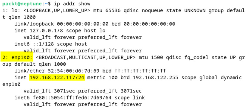
Figure 7.7 – Retrieving the current IP addresses with the ip command

We’ve highlighted some relevant information here, such as the network interface ID (2: enp1s0) and the IP address with the subnet prefix (192.168.122.117/24).

We’ll look at Ubuntu’s network configuration next. At the time of writing this book, the released version of Ubuntu is 22.04.2 LTS.

Ubuntu network configuration

Ubuntu 22.04 provides the netplan command-line utility for easy network configuration. netplan uses a YAML Ain’t Markup Language (YAML) configuration file to generate the network interface bindings. The netplan configuration file(s) is in the /etc/netplan/ directory, and we can access it by using the following command:

ls /etc/netplan/

In our case, the configuration file is 00-installer-config.yaml.

Changing the network configuration involves editing the netplan YAML configuration file. As good practice, we should always make a backup of the current configuration file before making changes. Changing a network configuration would most commonly involve setting up either a dynamic or a static IP address. We will show you how to configure both types in the next few sections. We’ll look at dynamic IP addressing first.

Dynamic IP configuration

To enable a dynamic (DHCP) IP address, we must edit the netplan configuration file and set the dhcp4 attribute to true (as shown in Figure 7.8) for the network interface of our choice (ens33, in our case). Open the 00-installer-config.yaml file with your text editor of choice (nano, in our case):

sudo nano /etc/netplan/00-installer-config.yaml

Here’s the related configuration excerpt, with the relevant points highlighted:

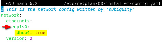
Figure 7.8 – Enabling DHCP in the netplan configuration

After saving the configuration file, we can test the related changes with the following command:

sudo netplan try

We’ll get the following response:

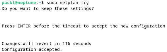
Figure 7.9 – Testing and accepting the netplan configuration changes

The netplan keyword validates the new configuration and prompts the user to accept the changes. The following command applies the current changes to the system:

sudo netplan apply

Next, we will configure a static IP address using netplan.

Static IP configuration

To set the static IP address of a network interface, we start by editing the netplan configuration YAML file, as follows:

sudo nano /etc/netplan/00-installer-config.yaml

Here’s a configuration example with a static IP address of 192.168.122.22/24:

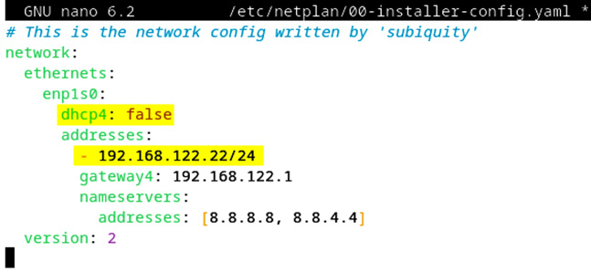
Figure 7.10 – Static IP configuration example with netplan

After saving the configuration, we can test and accept it, and then apply changes, as we did in the Dynamic IP section, with the following commands:

sudo netplan try
sudo netplan apply

For more information on the netplan command-line utility, see netplan --help or the related system manual (man netplan).

We’ll look at the Fedora network configuration next. At the time of writing, the current released version of Fedora is 37.

Fedora/RHEL network configuration

Starting with Fedora 33 and RHEL 9, network configuration files are no longer kept in the /etc/sysconfig/network-scripts/ directory. To learn more about the new configuration options, read the following file:

cat /etc/sysconfig/network-scripts/readme-ifcfg-rh.txt

The preferred method to configure the network in Fedora/RHEL is to use the nmcli utility. This location is deprecated and no longer used by NetworkManager in Fedora; it can still be used, but we do not recommend it. The new NetworkManager keyfiles are stored inside the /etc/NetworkManager/system-connections/ directory.

Let’s use some basic nmcli commands to view information about our connections. To learn about nmcli, read the related manual pages. First, let’s find information about our active connection using the following command:

nmcli connection show

The output will show basic information about the name of the connection, UUID, type, and the device used. The following screenshot shows the relevant information on our Fedora 37 VM:

Figure 7.11 – Using nmcli to view connection information

Similar to Ubuntu, when using Fedora/RHEL, changing a network configuration would most commonly involve setting up either a dynamic or a static IP address. We will show you how to configure both types in the following sections. Let’s look at dynamic IP addressing first.

Dynamic IP configuration

To configure a dynamic IP address using ncmli, we can run the following command:

sudo nmcli connection modify 'Wired connection 1' ipv4.method auto

The ipv4.method auto directive enables DHCP. There is no output from the command; after execution, you will be returned to the prompt again. You can check if the command worked by viewing the /etc/NetworkManager/system-connections/ directory. In our case, there is a new keyfile inside. It has the same name as our connection. The following is an excerpt:

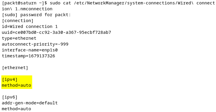
Figure 7.12 – New configuration keyfile

Next, we’ll configure a static IP address.

Static IP configuration

To perform the equivalent static IP address changes using ncmli, we need to run multiple commands. First, we must set the static IP address, as follows:

sudo nmcli connection modify 'Wired connection 1' ipv4.address 192.168.122.3/24

If no previous static IP address has been configured, we recommend saving the preceding change before proceeding with the next steps. The changes can be saved with the following code:

sudo nmcli connection down 'Wired connection 1'
sudo nmcli connection up 'Wired connection 1'

Next, we must set the gateway and DNS IP addresses, as follows:

sudo nmcli connection modify 'Wired connection 1' ipv4.gateway 192.168.122.1
sudo nmcli connection modify 'Wired connection 1' ipv4.dns 8.8.8.8

Finally, we must disable DHCP with the following code:

sudo nmcli connection modify 'Wired connection 1' ipv4.method manual

After making these changes, we need to restart the 'Wired connection 1' network interface with the following code:

sudo nmcli connection down 'Wired connection 1'
sudo nmcli connection up 'Wired connection 1'

Now, let’s see the results of all the commands we’ve performed. After bringing the connection up again, let’s check the new IP address and the contents of the network keyfile. The following figure shows the new IP we assigned to the system (192.168.122.3) by using the ip addr show command:

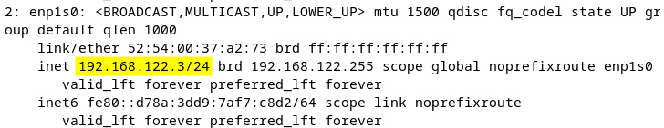
Figure 7.13 – Checking the new IP address

Now, let’s view the contents of the network keyfile to see the changes that were made for static IP configuration. Remember that the location of the file is /etc/NetworkManager/system-connections/:

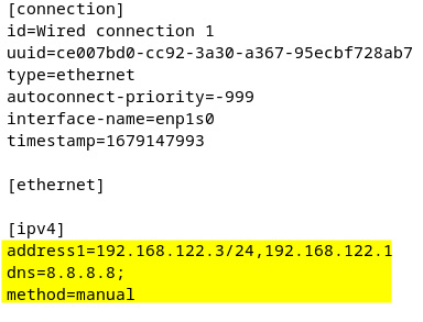
Figure 7.14 – New keyfile configuration for the static IP address

The nmcli utility is a powerful and useful one. At the end of this chapter, we will provide you with some useful links for learning more about it. Next, we’ll take a look at how to configure network services on openSUSE.

openSUSE network configuration

openSUSE provides several tools for network configuration: Wicked and NetworkManager. According to the official SUSE documentation, Wicked is used for all types of machines, from servers to laptops and workstations, whereas NetworkManager is used only for laptop and workstation setup and is not used for server setup. However, in openSUSE Leap, Wicked is set up by default on both desktop or server configurations, and NetworkManager is set up by default on laptop configurations.

For example, on our main workstation (which is a laptop), if we want to see which service is running by default on openSUSE Leap, we can use the following command:

sudo systemctl status network

The output will show us which service is running, and in our case, it is NetworkManager:

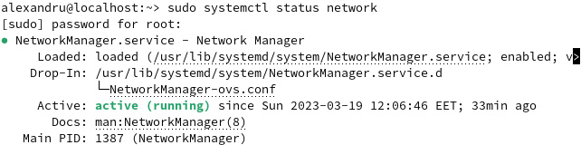
Figure 7.15 – Checking which network service is running in openSUSE

When running the same command inside an openSUSE Leap server VM, the result is different. The output shows that Wicked is running by default. The following screenshot shows an example:

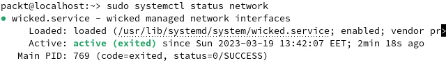
Figure 7.16 – Wicked is running inside the openSUSE server

As a result, we will perform all the examples in this section on an openSUSE Leap server VM, thus using Wicked as the default network configuration tool. In the next section, we will configure dynamic IP on an openSUSE machine.

Dynamic IP configuration

Before setting anything up, let’s check for active connections and devices. We can do this by using the following command:

wicked show all

The output will show all the active devices. The following screenshot shows an excerpt from the output on our machine:

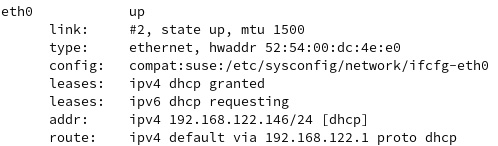
Figure 7.17 – Information about active devices

There are two active connections, one is loopback (lo) and the other is on the ethernet port (eth0). We will only show information related to eth0. The location where Wicked stores configuration files in openSUSE is /etc/sysconfig/network. If we do a listing of that directory, we will see that it is already populated with configuration files for existing connections:

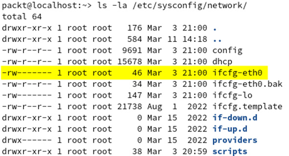
Figure 7.18 – Location of the Wicked configuration files

In our case, and maybe it will be the same for you, the file we are interested in is called ifcfg-eth0; we can open it with a text editor or concatenate it. Let’s take a look at the contents of the file:

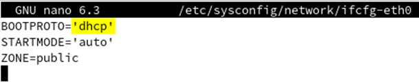
Figure 7.19 – Information provided by the configuration file

As shown in the preceding screenshot, the information provided is rather scarce but relevant. For a more detailed output, we can use the following command:

sudo wicked show-config

This will provide much more relevant information directly to the monitor. The following screenshot provides an excerpt from our output, with detailed IPv4 DHCP information:

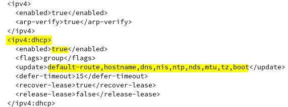
Figure 7.20 – Detailed information provided by Wicked

To better understand this output, we recommend reading the config file and, if available, the dhcp files inside the /etc/sysconfig/network directory. These files provide information about specific variables and default parameters needed for configuring the network devices.

Dynamic IP addresses are usually set up by default when installing the operating system. If yours is not configured, all you need to do is create a configuration file inside /etc/sysconfig/network and give it a relevant name based on the device you are using to connect to the network, such as ifcfg-eth0. Inside that file, you will have to provide just three lines, as seen in Figure 7.19. The following commands are needed for the actions described in this paragraph:

• Check your device name using the ip addr command:

  ip addr show

• Create a configuration file inside the /etc/sysconfig/network directory:

  sudo nano /etc/sysconfig/network/ifcfg-eth0

• Provide relevant information for the DHCP configuration:

  BOOTPROTO='dhcp'
  STARTMODE='auto'
  ZONE=public

• Restart the Wicked service:

  sudo systemctl restart wicked

• Check for connectivity by using either a web browser on your system or the ping command. Here’s an example:

  ping google.com

In the following section, we will show you how to set up a static IP configuration.

Static IP configuration

To set up a static IP configuration, you would need to manually provide variables for the configuration files. These files are the same ones that were presented in the previous section. The location of the files is /etc/sysconfig/network. For example, you can create a new file for the eth0 device connection and provide the information you want. Let’s look at an example of using our openSUSE Leap server VM. However, before doing this, we advise you to open the manual pages for the ifcfg utility as they provide valuable information on the variables used for this exercise.

Therefore, we will set the ifcfg configuration file as follows:

• First, we will check for the IP address and the network device name; in our case, the dynamically allocated IP is 192.168.122.146 and the device’s name is eth0:

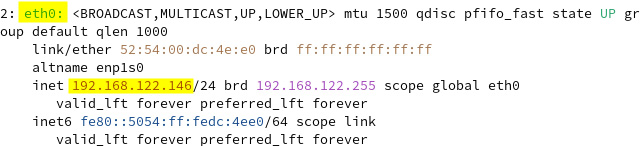
Figure 7.21 – IP and device information

• Go to the /etc/sysconfig/network directory and edit the ifcfg-eth0 file; we will use the following variables for static IP configuration:
  • BOOTPROTO='static': This allows us to use a fixed IP address that will be provided by using the IPADDR variable
  • STARTMODE='auto': The interface will be automatically enabled on boot
  • IPADDR='192.168.122.144': The IP address we choose for the machine
  • ZONE='public': The zone used by the firewalld utility
  • PREFIXLEN='24': The number of bits in the IPADDR variable

  This will look as follows:

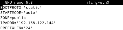
Figure 7.22 – New variables for static IP configuration

• Save the changes to the new file and restart the Wicked daemon:

  sudo systemctl restart wickedd.service

• Enable the interface so that the changes appear:

  sudo wicked ifup eth0

• Run the ip addr show command again to check for the new IP address:

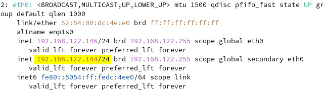
Figure 7.23 – New IP address assigned to eth0

At this point, you know how to configure networking devices in all major Linux distributions, using their preferred utilities. We’ve merely scratched the surface of this matter, but we’ve provided sufficient information for you to start working with network interfaces in Linux. For more information, feel free to read the manual pages freely provided with your operating system. In the next section, we will approach the matter of hostname configuration.

Hostname configuration

To retrieve the current hostname on a Linux machine, we can use either the hostname or hostnamectl command, as follows:

hostname

The most convenient way to change the hostname is with the hostnamectl command. We can change the hostname to earth using the set-hostname parameter of the command:

sudo hostnamectl set-hostname earth

Let’s verify the hostname change with the hostname command again. You could use the hostnamectl command to verify the hostname. The output of the hostnamectl command provides more detailed information compared to the hostname command, as shown in the following screenshot:

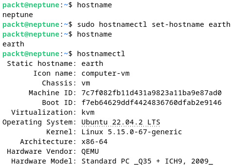
Figure 7.24 – Retrieving the current hostname with the different commands

Alternatively, we can use the hostname command to change the hostname temporarily, as follows:

sudo hostname jupiter

However, this change will not survive a reboot unless we also change the hostname in the /etc/hostname and /etc/hosts files. When editing these two files, change your hostname accordingly. The following screenshot shows the succession of commands:

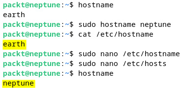
Figure 7.25 – The /etc/hostname and /etc/hosts files

After the hostname reconfiguration, a logout followed by a login would usually reflect the changes. Hostnames are important for coherent network management, where each system on the network should have relevant hostnames set up. In the following section, you’ll learn about network services in Linux.