Bagging – building an ensemble of classifiers from bootstrap samples

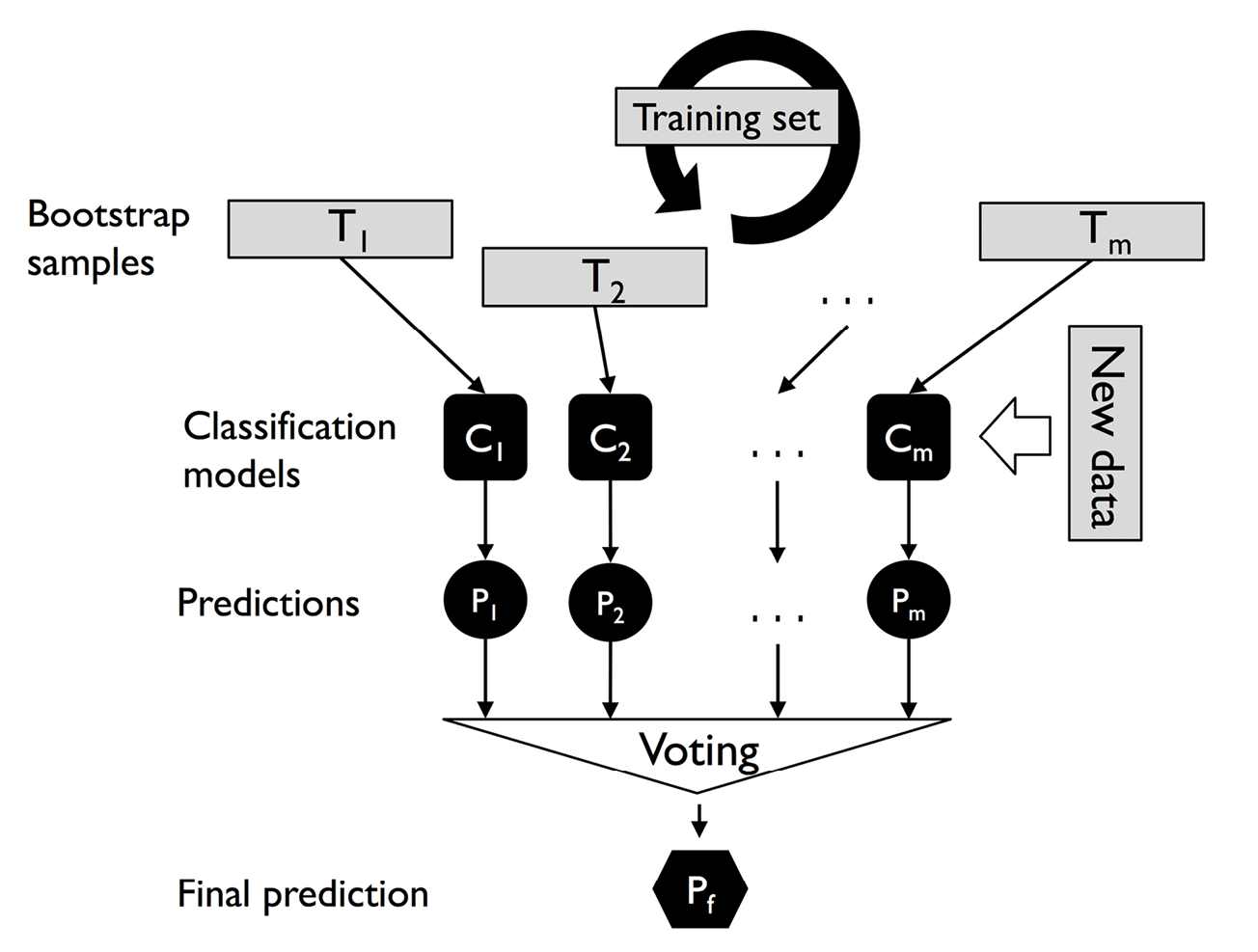
Bagging is an ensemble learning technique that is closely related to the MajorityVoteClassifier that we implemented in the previous section. However, instead of using the same training dataset to fit the individual classifiers in the ensemble, we draw bootstrap samples (random samples with replacement) from the initial training dataset, which is why bagging is also known as bootstrap aggregating.

The concept of bagging is summarized in Figure 7.6:

Figure 7.6: The concept of bagging

In the following subsections, we will work through a simple example of bagging by hand and use scikit-learn for classifying wine examples.

Bagging in a nutshell

To provide a more concrete example of how the bootstrap aggregating of a bagging classifier works, let’s consider the example shown in Figure 7.7. Here, we have seven different training instances (denoted as indices 1-7) that are sampled randomly with replacement in each round of bagging. Each bootstrap sample is then used to fit a classifier, C_j, which is most typically an unpruned decision tree:

Figure 7.7: An example of bagging

As you can see from Figure 7.7, each classifier receives a random subset of examples from the training dataset. We denote these random samples obtained via bagging as Bagging round 1, Bagging round 2, and so on. Each subset contains a certain portion of duplicates and some of the original examples don’t appear in a resampled dataset at all due to sampling with replacement. Once the individual classifiers are fit to the bootstrap samples, the predictions are combined using majority voting.

Note that bagging is also related to the random forest classifier that we introduced in Chapter 3. In fact, random forests are a special case of bagging where we also use random feature subsets when fitting the individual decision trees.

Model ensembles using bagging

Bagging was first proposed by Leo Breiman in a technical report in 1994; he also showed that bagging can improve the accuracy of unstable models and decrease the degree of overfitting. We highly recommend that you read about his research in Bagging predictors by L. Breiman, Machine Learning, 24(2):123–140, 1996, which is freely available online, to learn more details about bagging.

Applying bagging to classify examples in the Wine dataset

To see bagging in action, let’s create a more complex classification problem using the Wine dataset that was introduced in Chapter 4, Building Good Training Datasets – Data Preprocessing. Here, we will only consider the Wine classes 2 and 3, and we will select two features – Alcohol and OD280/OD315 of diluted wines:

>>> import pandas as pd
>>> df_wine = pd.read_csv('https://archive.ics.uci.edu/ml/'
...                       'machine-learning-databases/'
...                       'wine/wine.data',
...                       header=None)
>>> df_wine.columns = ['Class label', 'Alcohol',
...                    'Malic acid', 'Ash',
...                    'Alcalinity of ash',
...                    'Magnesium', 'Total phenols',
...                    'Flavanoids', 'Nonflavanoid phenols',
...                    'Proanthocyanins',
...                    'Color intensity', 'Hue',
...                    'OD280/OD315 of diluted wines',
...                    'Proline']
>>> # drop 1 class
>>> df_wine = df_wine[df_wine['Class label'] != 1]
>>> y = df_wine['Class label'].values
>>> X = df_wine[['Alcohol',
...              'OD280/OD315 of diluted wines']].values

Next, we will encode the class labels into binary format and split the dataset into 80 percent training and 20 percent test datasets:

>>> from sklearn.preprocessing import LabelEncoder
>>> from sklearn.model_selection import train_test_split
>>> le = LabelEncoder()
>>> y = le.fit_transform(y)
>>> X_train, X_test, y_train, y_test =\
...            train_test_split(X, y,
...                             test_size=0.2,
...                             random_state=1,
...                             stratify=y)

Obtaining the Wine dataset

You can find a copy of the Wine dataset (and all other datasets used in this book) in the code bundle of this book, which you can use if you are working offline or the UCI server at https://archive.ics.uci.edu/ml/machine-learning-databases/wine/wine.data is temporarily unavailable. For instance, to load the Wine dataset from a local directory, take the following lines:

df = pd.read_csv('https://archive.ics.uci.edu/ml/'
                 'machine-learning-databases'
                 '/wine/wine.data',
                 header=None)

and replace them with these:

df = pd.read_csv('your/local/path/to/wine.data',
                 header=None)

A BaggingClassifier algorithm is already implemented in scikit-learn, which we can import from the ensemble submodule. Here, we will use an unpruned decision tree as the base classifier and create an ensemble of 500 decision trees fit on different bootstrap samples of the training dataset:

>>> from sklearn.ensemble import BaggingClassifier
>>> tree = DecisionTreeClassifier(criterion='entropy',
...                               random_state=1,
...                               max_depth=None)
>>> bag = BaggingClassifier(base_estimator=tree,
...                         n_estimators=500,
...                         max_samples=1.0,
...                         max_features=1.0,
...                         bootstrap=True,
...                         bootstrap_features=False,
...                         n_jobs=1,
...                         random_state=1)

Next, we will calculate the accuracy score of the prediction on the training and test datasets to compare the performance of the bagging classifier to the performance of a single unpruned decision tree:

>>> from sklearn.metrics import accuracy_score
>>> tree = tree.fit(X_train, y_train)
>>> y_train_pred = tree.predict(X_train)
>>> y_test_pred = tree.predict(X_test)
>>> tree_train = accuracy_score(y_train, y_train_pred)
>>> tree_test = accuracy_score(y_test, y_test_pred)
>>> print(f'Decision tree train/test accuracies '
...       f'{tree_train:.3f}/{tree_test:.3f}')
Decision tree train/test accuracies 1.000/0.833

Based on the accuracy values that we printed here, the unpruned decision tree predicts all the class labels of the training examples correctly; however, the substantially lower test accuracy indicates high variance (overfitting) of the model:

>>> bag = bag.fit(X_train, y_train)
>>> y_train_pred = bag.predict(X_train)
>>> y_test_pred = bag.predict(X_test)
>>> bag_train = accuracy_score(y_train, y_train_pred)
>>> bag_test = accuracy_score(y_test, y_test_pred)
>>> print(f'Bagging train/test accuracies '
...       f'{bag_train:.3f}/{bag_test:.3f}')
Bagging train/test accuracies 1.000/0.917

Although the training accuracies of the decision tree and bagging classifier are similar on the training dataset (both 100 percent), we can see that the bagging classifier has a slightly better generalization performance, as estimated on the test dataset. Next, let’s compare the decision regions between the decision tree and the bagging classifier:

>>> x_min = X_train[:, 0].min() - 1
>>> x_max = X_train[:, 0].max() + 1
>>> y_min = X_train[:, 1].min() - 1
>>> y_max = X_train[:, 1].max() + 1
>>> xx, yy = np.meshgrid(np.arange(x_min, x_max, 0.1),
...                      np.arange(y_min, y_max, 0.1))
>>> f, axarr = plt.subplots(nrows=1, ncols=2,
...                         sharex='col',
...                         sharey='row',
...                         figsize=(8, 3))
>>> for idx, clf, tt in zip([0, 1],
...                         [tree, bag],
...                         ['Decision tree', 'Bagging']):
...     clf.fit(X_train, y_train)
...
...     Z = clf.predict(np.c_[xx.ravel(), yy.ravel()])
...     Z = Z.reshape(xx.shape)
...     axarr[idx].contourf(xx, yy, Z, alpha=0.3)
...     axarr[idx].scatter(X_train[y_train==0, 0],
...                        X_train[y_train==0, 1],
...                        c='blue', marker='^')
...     axarr[idx].scatter(X_train[y_train==1, 0],
...                        X_train[y_train==1, 1],
...                        c='green', marker='o')
...     axarr[idx].set_title(tt)
>>> axarr[0].set_ylabel('OD280/OD315 of diluted wines', fontsize=12)
>>> plt.tight_layout()
>>> plt.text(0, -0.2,
...          s='Alcohol',
...          ha='center',
...          va='center',
...          fontsize=12,
...          transform=axarr[1].transAxes)
>>> plt.show()

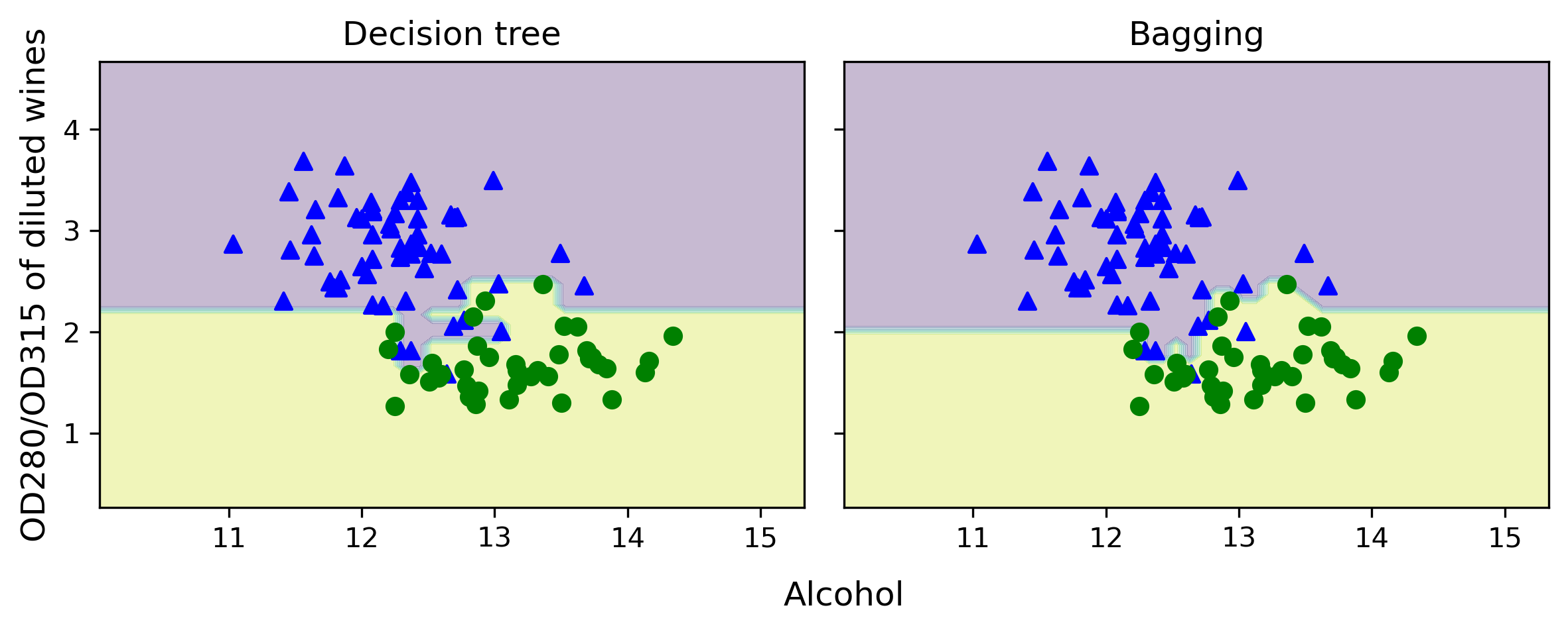
As we can see in the resulting plot, the piece-wise linear decision boundary of the three-node deep decision tree looks smoother in the bagging ensemble:

Figure 7.8: The piece-wise linear decision boundary of a decision tree versus bagging

We only looked at a very simple bagging example in this section. In practice, more complex classification tasks and a dataset’s high dimensionality can easily lead to overfitting in single decision trees, and this is where the bagging algorithm can really play to its strengths. Finally, we must note that the bagging algorithm can be an effective approach to reducing the variance of a model. However, bagging is ineffective in reducing model bias, that is, models that are too simple to capture the trends in the data well. This is why we want to perform bagging on an ensemble of classifiers with low bias, for example, unpruned decision trees.