So far, we have studied derivatives, which is a method for extracting information about the rate of change of a function. But as you may have realized, integration is the reverse of the earlier problems.
In integration, we find the area underneath a curve. For example, if we have a car and our function gives us its velocity, the area under the curve will give us the distance it has traveled between two points.
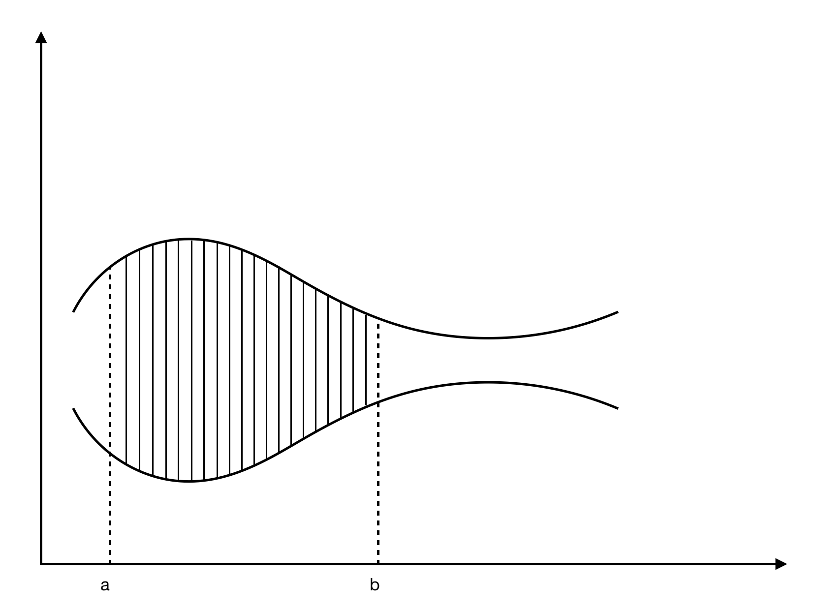
Let's suppose we have the curve  , and the area under the curve between x = a (the lower limit) and x = b (the upper limit, also written as [a, b]) is S. Then, we have the following:
The diagramatical representation of the curve is as follows:
This can also be written as follows:
In the preceding function, the following applies:  , and
, and  is in the subinterval
  .
.
The function looks like this:
The integral gives us an approximation of the area under the curve such that for some, ε > 0 (ε is assumed to be a small value), the following formula applies:
Now, let's suppose our function lies both above and below the x axis, thus taking on positive and negative values, like so:
As we can see from the preceding screenshot, the portions above the x axis (A1) have a positive area, and the portions below the x axis (A2) have a negative area. Therefore, the following formula applies:
Working with sums is an important part of evaluating integrals, and understanding this requires some new rules for sums. Look at the following examples:
Now, let's explore some of the important properties of integrals, which will help us as we go deeper into the chapter. Look at the following examples:

 , when
 , where c is a constant


Now, suppose we have the function  , which looks like this:
Then, we get the following property:
This property only works for functions that are continuous and have adjacent intervals.


 value tells us whether the line is moving upward or downward.
 value tells us by how much the line is above or below the origin.
  . After having found the value for m, we find the value of b by using the line equation and plugging into it the value for m and one (x, y) point on the line, and solve for b.

 have to do with this? This tells us that we want the two points on the curve to be as close to each other as possible so that when we are sketching the gradient on the curve, it looks like a straight line at one point on the curve. This allows us to better visualize and understand the effect of the change, as can be seen in the following screenshot:


 and
and  .
.  , is the same as this one:
 .
.

 or
or  —that are not as straightforward as the ones we saw earlier. The function
  is not differentiable at x = 0 because its value is undefined. This is known as discontinuity.
 ; however, e (known as Euler's number) has a very interesting property whereby the function is equal to its derivative—that is,
  .
.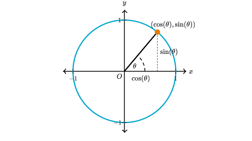
 and cosine is
 .
. , then
  . However, if
  , then
  .
. 
 , then f(x) is increasing at x = t.
 , then f(x) is decreasing at x = t
 , then x=t is a critical point of f(x).
 . The derivative of this function is shown here:
 or
or  . As before, where the first derivative told us whether the function was increasing or decreasing, the second derivative gives us the same information about the first derivative—whether it is increasing or decreasing.
  , then f(x) is concave up at x=t.
 , then f(x) is concave down at x=t
 , then at x=t we obtain no new information about f(x).
 and
and  , then f(x) has a local minimum at x=t.
 and
and  , then f(x) has a local maximum at x=t
 and
and  , then at x=t we learn nothing new about f(x).
 . The derivative is
  .
. 

 , which is the same as before.
 . The derivative is
 and
and  . Then, we have the following:

 , which is often written as
  and read as f of g of x. This means that the output of g(x) will become the input to the function f.
 .
.  and
and  . We then differentiate the two functions and get
  and
and  .
. .
. 


 , then
  (where c is some constant), from which we can confirm that
  .
. 


 .
. and
and  and
and 


 ; therefore,
 ; therefore,


 .
.
 , and the differential of u is then
  . This changes the problem into the following:

 , we get the following:

 , then the following applies:


 merely states that we plug in the value b in place of x and evaluate it, and then subtract it from the evaluation at a.
 and
and  ; then, the differentials are
  and
and  . And so, the formula becomes this: