Transforming data to fit analytic needs

In the previous section, you learned how to extract data and import it into R from various sources. Now you can transform it to create subsets of the data. This is useful to provide other team members with a portion of the data they can use in their work without requiring the complete dataset. In this section, you will learn the following four key activities associated with transformation:

• Filtering data rows

• Selecting data columns

• Adding a calculated column from existing data

• Aggregating data into groups

You will learn how to use functions from the dplyr package to perform data manipulation. If you are familiar with SQL, then dplyr is similar in how it filters, selects, sorts, and groups data. If you are not familiar with SQL, do not worry. This section will introduce you to the dplyr package. Learn more about the dplyr package by typing browseVignettes(package = "dplyr") into your R console.

Note

Request from marketing: Marketing would like an extract from the data with revenues during the spring and summer seasons from days when only casual users rent bikes. They want a small CSV file with just the number of casual renters and revenue grouped by season.

Filtering data rows

You will filter rows with dplyr using the filter() function to extract a subset of rows that meet the criteria defined with logical operators such as those shown in the following table (RStudio, 2015). Read more about this by typing ?Comparison or ?base::Logic in the R console:

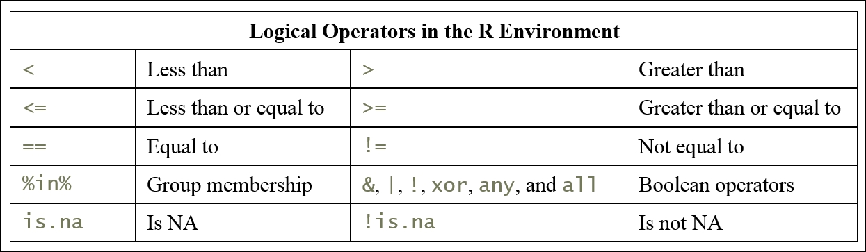
You can use these operators to pass a criterion, or many criteria, into your filter. Marketing would like to know how many times during spring or summer that only casual users rented bikes. You can begin creating a subset of the data by using the filter() function along with the == operator and the or Boolean ( | ). Place the results in a temporary extracted_rows data frame:

library(dplyr) 
extracted_rows <- filter(bike, registered == 0,  
                         season == 1 | season == 2) 
dim(extracted_rows) 

We get the following output:

[1] 10 12

The dim() function call shows only 10 observations meet the filter criteria. This demonstrates the power of filtering larger datasets.

There are various ways of transforming the data. You can create an identical dataset using the %in% operator. This operator looks at each row (observation) and determines whether it is a member of the group based on criteria you specify. The first parameter is the name of the data frame, the second and successive parameters are filtering expressions:

using_membership <- filter(bike, registered == 0, season %in% c(1, 2)) 
identical(extracted_rows, using_membership) 

We get the output as follows:

[1] TRUE

The identical() function compares any two R objects and returns TRUE if they are identical and FALSE otherwise. You created a subset of data by filtering rows and saving it in a separate data frame. Now you can select columns from that.

Selecting data columns

The select() function extracts columns you desire to retain in your final dataset. The marketing team indicated they were only interested in the season and casual renters. They did not express interest in environmental conditions or holidays. Providing team members data products that meet their specification is an important way to sustain relationships.

You can extract the required columns from extracted_rows and save these in another temporary extracted_columns data frame. Pass the select() function, data frame, and names of the columns to extract, season and casual:

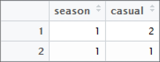
extracted_columns <- select(extracted_rows, season, casual) 

The following table provides a view of the first two observations from the subset data frame you generated. You notice that there is something missing. Marketing wants to know the number of casual renters and revenue by season. There is no revenue variable in the data you are using. What can you do about this? You can add a column to the data frame, as described in the following section:

Adding a calculated column from existing data

For your particular situation, you will be adding a calculated column. You asked marketing about the structure of rental costs and learn that casual renters pay five dollars for a day pass. You figured out that all you have to do is multiply the number of casual renters by five to get the revenues for each day in your data frame.

The mutate() function will calculate and add one or more columns, depending on the parameters. Your parameters include the data frame and an expression indicating the name of the new column and the calculation to create the revenue:

add_revenue <- mutate(extracted_columns, revenue = casual * 5) 

The output will be as follows:

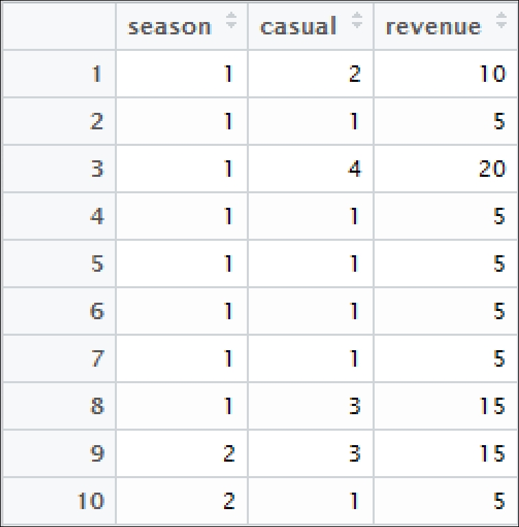
Perfect! You are nearly done. All you have left to do is to group and summarize the data into a final data frame.

Aggregating data into groups

The dplyr package provides you the group_by() and summarise() functions to help you aggregate data. You will often see these two functions used together. The group_by() function takes the data frame and variable on which you would like to group the data as parameters, in your case, season:

grouped <- group_by(add_revenue, season) 

The summarise() function takes the data frame and all the variables you want to summarize as parameters. This also requires you to specify how you would like to summarize them. You may chose an average, minimum, maximum, or sum. Marketing wants to know total rentals and revenue by season, so you will use the sum() function:

report <- summarise(grouped, sum(casual), sum(revenue)) 

We get the output as follows:

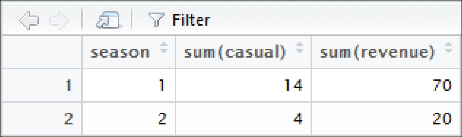
This looks like it is what the marketing group wants. Now you have to deliver it.

Tip

R tip: There are many other transformation functions provided by the dplyr package. You can type ??dplyr in your R console to get more information.