Understanding decision trees

A decision tree is a very good example of "divide and conquer". It is one of the most practical and widely used methods for inductive inference. It is a supervised learning method that can be used for both classification and regression. It is non-parametric and its aim is to learn by inferring simple decision rules from the data and create such a model that can predict the value of the target variable.

Before taking a decision, we analyze the probability of the pros and cons by weighing the different options that we have. Let's say we want to purchase a phone and we have multiple choices in the price segment. Each of the phones has something really good, and maybe better than the other. To make a choice, we start by considering the most important feature that we want. And as such, we create a series of features that it has to pass to become the ultimate choice.

In this section, we will learn about:

• Decision trees
• Entropy measures
• Random forests

We will also learn about famous decision tree learning algorithms such as ID3 and C5.0.

Building decision trees – divide and conquer

A heuristic called recursive partitioning is used to build decision trees. In this approach, our data is split into similar classes of smaller and smaller subsets as we move along.

A decision tree is actually an inverted tree. It starts from the root and ends up at the leaf nodes, which are the terminal nodes. The splitting of the node into branches is based on logical decisions. The whole dataset is represented at the root node. A feature is chosen by the algorithm that is most predictive of the target class. Then it partitions the examples into distinct value groups of this particular feature. This represents the first set of the branches of our tree.

The divide-and-conquer approach is followed until the end point is reached. At each step, the algorithm continues to choose the best candidate feature.

The end point is defined when:

• At a particular node, nearly all the examples belong to the same class
• The feature list is exhausted
• A predefined size limit of the tree is reached

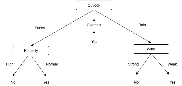
The preceding image is a very famous example of decision tree. Here, a decision tree is made to find out whether to go out or not:

• Outlook is the root node. This refers to all the possible classes of the environment
• Sunny, overcast, and Rain are the branches.
• Humidity and Wind are the leaf nodes, which are again split into branches, and a decision is taken depending on the favorable environment.

These trees can also be re-represented as if-then rules, which would be easily understandable. Decision trees are one of the very successful and popular algorithms, with a broad range of applications.

The following are some of the applications of decision trees:

• Decision of credit card / loan approval: Credit scoring models are based on decision trees, where every applicant's information is fed to decide whether a credit card / loan should be approved or not.
• Medical diagnosis: Various diseases are diagnosed using well-defined and tested decision trees based on symptoms, measurements, and tests.

Where should we use decision tree learning?

Although there are various decision tree learning methods that can be used for a variety of problems, decision trees are best suited for the following scenarios:

• Attribute-value pairs are scenarios where instances are described by attributes from a fixed set and values. In the previous example, we had the attribute as "Wind" and the values as "Strong" and "Weak". These disjoint possible values make it easy to create decision tree learning, although attributes with real values can also be used.
• The final output of the target function has a discreet value, like the previous example, where we had "Yes" or "No". The decision tree algorithm can be extended to have more than two possible target values. Decision trees can also be extended to have real values as outputs, but this is rarely used.
• The decision tree algorithm is robust to errors in the training dataset. These errors can be in the attribute values of the examples or the classification of the examples or both.
• Decision tree learning is also suited for missing values in a dataset. If the values are missing in some examples where they are available for attributes in other examples, then decision trees can be used.

Advantages of decision trees

• It is easy to understand and interpret decision trees. Visualizing decision trees is easy too.
• In other algorithms, data normalization needs to be done before they can be applied. Normalization refers to the creation of dummy variables and removing blank values. Decision trees, on the other hand, require very less data preparation.
• The cost involved in prediction using a decision tree is logarithmic with respect to the number of examples used in training the tree.
• Decision trees, unlike other algorithms, can be applied to both numerical and categorical data. Other algorithms are generally specialized to be used for only one type of variable.
• Decision trees can easily take care of the problems where multiple outputs is a possibility.
• Decision trees follow the white box model, which means a condition is easily explained using Boolean logic if the situation is observable in the model. On the other hand, results are comparatively difficult to interpret in a black box model, such as artificial neural networks.
• Statistical tests can be used to validate the model. Therefore, we can test the reliability of the model.
• It is able to perform well even if there is a violation in the assumptions from the true model that was the source of the data.

Disadvantages of decision trees

We've covered where decision trees are suited and their advantages. Now we will go through the disadvantages of decision trees:

• There is always a possibility of overfitting the data in decision trees. This generally happens when we create trees that are over-complex and are not possible to generalize well.
• To avoid this, various steps can be taken. One method is pruning. As the name suggests, it is a method where we set the maximum depth to which the tree can grow.
• Instability is always a concern with decision trees as a small variation in the data can result in generation of a different tree altogether.
• The solution to such a scenario is ensemble learning, which we will study in the next chapter.
• Decision tree learning may sometimes lead to the creation of biased trees, where some classes are dominant over others. The solution to such a scenario is balancing the dataset prior to fitting it to the decision tree algorithm.
• Decision tree learning is known to be NP-complete, considering several aspects of optimality. This holds even for the basic concepts.
• Usually, heuristic algorithms like greedy algorithms are used where a locally optimal decision is made at each node. This doesn't guarantee that we will have a decision tree that is globally optimal.
• Learning can be hard for the concepts such as Parity, XOR, and multiplexer problems, where decision trees cannot represent them easily.

Decision tree learning algorithms

There are various decision tree learning algorithms that are actually variations of the core algorithm. The core algorithm is actually a top-down, greedy search through all possible trees.

We are going to discuss two algorithms:

• ID3
• C4.5 and C5.0

The first algorithm, ID3 (Iterative Dichotomiser 3), was developed by Ross Quinlan in 1986. The algorithm proceeds by creating a multiway tree, where it uses a greedy search to find each node and the features that can yield maximum information gain for the categorical targets. As trees can grow to the maximum size, which can result in over-fitting of data, pruning is used to make the generalized model.

C4.5 came after ID3 and eliminated the restriction that all features must be categorical. It does this by defining dynamically a discrete attribute based on the numerical variables. This partitions into a discrete set of intervals from the continuous attribute value. C4.5 creates sets of if-then rules from the trained trees of the ID3 algorithm. C5.0 is the latest version; it builds smaller rule sets and uses comparatively lesser memory.

How a decision tree algorithm works

The decision tree algorithm constructs the top-down tree. It follows these steps:

1. To know which element should come at the root of the tree, a statistical test is done on each instance of the attribute to determine how well the training examples can be classified using this attribute alone.
2. This leads to the selection of the best attribute at the root node of the tree.
3. Now at this root node, for each possible value of the attribute, the descendants are created.
4. The examples in our training dataset are sorted to each of these descendant nodes.
5. Now for these individual descendant nodes, all the previous steps are repeated for the remaining examples in our training dataset.
6. This leads to the creation of an acceptable tree for our training dataset using a greedy search. The algorithm never backtracks, which means it never reconsiders the previous choices and follows the tree downwards.

Understanding and measuring purity of node

The decision tree is built top-down. It can be tough to decide on which attribute to split on each node. Therefore, we find the feature that best splits the target class. Purity is the measure of a node containing only one class.

Purity in C5.0 is measured using entropy. The entropy of the sample of the examples is the indication of how class values are mixed across the examples:

• 0: The minimum value is an indication of the homogeneity in the class values in the sample
• 1: The maximum value is an indication that there is maximum amount of disorder in the class values in the sample

Entropy is given by:

In the preceding formula, S refers to the dataset that we have and c refers to the class levels. For a given class i, p is the proportion of the values.

When the purity measure is determined, the algorithm has to decide on which feature the data should be split. To decide this, the entropy measure is used by the algorithm to calculate how the homogeneity differs on splitting on each possible feature. This particular calculation done by the algorithm is the information gain:

The difference between the entropy before splitting the dataset (S1) and the resulting partitions from splitting (S2) is called information gain (F).

An example

Let's apply what we've learned to create a decision tree using Julia. We will be using the example available for Python on http://scikit-learn.org/ and Scikitlearn.jl by Cedric St-Jean.

We will first have to add the required packages:

julia> Pkg.update() 
julia> Pkg.add("DecisionTree") 
julia> Pkg.add("ScikitLearn") 
julia> Pkg.add("PyPlot") 

ScikitLearn provides the interface to the much-famous library of machine learning for Python to Julia:

julia> using ScikitLearn 
julia> using DecisionTree 
julia> using PyPlot 

After adding the required packages, we will create the dataset that we will be using in our example:

julia> # Create a random dataset 
julia> srand(100) 
julia> X = sort(5 * rand(80)) 
julia> XX = reshape(X, 80, 1) 
julia> y = sin(X) 
julia> y[1:5:end] += 3 * (0.5 - rand(16)) 

This will generate a 16-element Array{Float64,1}.

Now we will create instances of two different models. One model is where we will not limit the depth of the tree, and in other model, we will prune the decision tree on the basis of purity:

We will now fit the models to the dataset that we have. We will fit both the models.

This is the first model. Here our decision tree has 25 leaf nodes and a depth of 8.

This is the second model. Here we prune our decision tree. This has 6 leaf nodes and a depth of 4.

Now we will use the models to predict on the test dataset:

julia> # Predict 
julia> X_test = 0:0.01:5.0 
julia> y_1 = predict(regr_1, hcat(X_test)) 
julia> y_2 = predict(regr_2, hcat(X_test)) 

This creates a 501-element Array{Float64,1}.

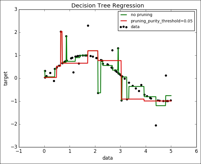
To better understand the results, let's plot both the models on the dataset that we have:

julia> # Plot the results 
julia> scatter(X, y, c="k", label="data") 
julia> plot(X_test, y_1, c="g", label="no pruning", linewidth=2) 
julia> plot(X_test, y_2, c="r", label="pruning_purity_threshold=0.05", linewidth=2) 
 
julia> xlabel("data") 
julia> ylabel("target") 
julia> title("Decision Tree Regression") 
julia> legend(prop=Dict("size"=>10)) 

Decision trees can tend to overfit data. It is required to prune the decision tree to make it more generalized. But if we do more pruning than required, then it may lead to an incorrect model. So, it is required that we find the most optimized pruning level.

It is quite evident that the first decision tree overfits to our dataset, whereas the second decision tree model is comparatively more generalized.